Ignore data within parentheses from formula

[Niall19]

Hello,

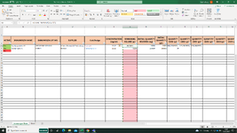
So, I'm quite the novice when it comes to excel formulae so any help would be greatly appreciated. This is probably very straightforward but I would like "Remaining volume" in cell "G3" to substract the values in "J3", "K3" and "L3" from the value in "I3", crucially, ignoring the data within the parentheses. Is this possible and if so, could a kind soul offer some advice on how to achieve this?

REMAINING VOLUME (µL)	INITIAL QUANTITY RECEIVED (mg)	INITIAL QUANTITY (µL)	QUANTITY USED (µL)	QUANTITY USED (µL)	QUANTITY USED (µL)
SUM of initial quantity minus all quantity used, ignoring parentheses.	10000​	10000​	100 (19SEP22)	127 (23SEP22)	120 (26SEP22)
G3^​	H3^​	I3^​	J3^​	K3^	L3 ^
​
​

Kind regards,
Niall

 

[Fluff]

Hi & welcome to MrExcel.
How about

Fluff.xlsm
	G	H	I	J	K	L
1
2	REMAINING VOLUME (µL)	INITIAL QUANTITY RECEIVED (mg)	INITIAL QUANTITY (µL)	QUANTITY USED (µL)	QUANTITY USED (µL)	QUANTITY USED (µL)
3	9653	10000	10000	100 (19SEP22)	127 (23SEP22)	120 (26SEP22)
Data

Cell Formulas
Range	Formula
G3	G3	=I3-SUM(--TEXTSPLIT(J3:L3,"("))

 

[Niall19]

Hi & welcome to MrExcel.
How about

Fluff.xlsm
	G	H	I	J	K	L
1
2	REMAINING VOLUME (µL)	INITIAL QUANTITY RECEIVED (mg)	INITIAL QUANTITY (µL)	QUANTITY USED (µL)	QUANTITY USED (µL)	QUANTITY USED (µL)
3	9653	10000	10000	100 (19SEP22)	127 (23SEP22)	120 (26SEP22)
Data

Cell Formulas
Range	Formula
G3	G3	=I3-SUM(--TEXTSPLIT(J3:L3,"("))

Hi,
Thank you for the assistance! I've tried this formula but unfortunately it's throwing up a "#NAME?" error. I'm sure this is something I am doing wrong. Any ideas as to what that might be?

Niall

 

[fjns]

Hi, try this formula for G3

=I3-IF(IFERROR(SEARCH("(",J3),0)=0,J3,LEFT(J3,SEARCH("(",J3)-1))-IF(IFERROR(SEARCH("(",K3),0)=0,K3,LEFT(K3,SEARCH("(",K3)-1))-IF(IFERROR(SEARCH("(",L3),0)=0,L3,LEFT(L3,SEARCH("(",L3)-1))

 

[Fluff]

I'm sure this is something I am doing wrong

Nope, you probably don't have the Textsplit function yet.
How about

=I3-SUM(FILTERXML("<k><m>"&TEXTJOIN("</m><m>",,SUBSTITUTE(J3:L3," ","</m><m>"))&"</m></k>","//m"))

 

[Niall19]

Nope, you probably don't have the Textsplit function yet.
How about

=I3-SUM(FILTERXML("<k><m>"&TEXTJOIN("</m><m>",,SUBSTITUTE(J3:L3," ","</m><m>"))&"</m></k>","//m"))

This is really cool! Thank you so much for this solution.

Take care!

 

[Fluff]

Glad we could help & thanks for the feedback.

 

[Niall19]

Glad we could help & thanks for the feedback.

Just one more thing which would be great to find a solution for, not a requirement but it would tidy up the appearance of the spreadsheet - The formula/column "G" cells which are blank (no entries made yet) are showing up the "#VALUE!" error message.

Would there be a way to write something into the formula to show these cells as blank or 0 when they haven't yet been filled in, but still have the formula applied in advance? Sorry for another novice level question!

Kind regards,
Niall

 

[Sufiyan97]

Try

=IFERROR(I3-SUM(FILTERXML("<k><m>"&TEXTJOIN("</m><m>",,SUBSTITUTE(J3:L3," ","</m><m>"))&"</m></k>","//m")),"")

 

[fjns]

Hi, try this formula for G3

=IF(OR(ISBLANK(I3),ISBLANK(J3),ISBLANK(K3),ISBLANK(L3)),0,I3-IF(IFERROR(SEARCH("(",J3),0)=0,J3,LEFT(J3,SEARCH("(",J3)-1))-IF(IFERROR(SEARCH("(",K3),0)=0,K3,LEFT(K3,SEARCH("(",K3)-1))-IF(IFERROR(SEARCH("(",L3),0)=0,L3,LEFT(L3,SEARCH("(",L3)-1)))