Index and Match Excel Question.

[DNapoli]

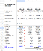
Tab1 "01.31.2021" has a "Total" line in column B. I want to return the values in columns C, D, E ,F,G, and H from the "Total Line" in my second tab.
Tab2 "Metrics V3" starts in column L 17 and goes down. I want to populate the totals from the 1st sheet into the 2nd sheet (Metrics V3)
My formula does not drag down in the 2nd sheet. I had to edit it to get it to work manually. What am I doing incorrectly?
=INDEX('01.31.2021'!$C:$H, MATCH("Total", '01.31.2021'!$B:$B, 0) + ROW() - ROW($L$17), COLUMN() - COLUMN($L$17) + 1)
=INDEX('01.31.2021'!$C:$H, MATCH("Total", '01.31.2021'!$B:$B, 0) + ROW(L18) - ROW($L$18), COLUMN() - COLUMN($L$18) + 2)
=INDEX('01.31.2021'!$C:$H, MATCH("Total", '01.31.2021'!$B:$B, 0) + ROW(L19) - ROW($L$19), COLUMN() - COLUMN($L$19) + 3)
View attachment 108883

01.31.2021 Tab

Metrics V3 Tab

 

[DNapoli]

.. provided '01.31.2021' only has one "Total" row. Also, filter on an entire column like that is relatively slow compared to a MATCH type function.

This would be my suggestion for L17 on 'Metrics V3'

=TRANSPOSE(INDEX('01.31.2021'!C:H,XMATCH("Total",'01.31.2021'!B:B),0))

Thank you Peter!! I will try this.

 

[DNapoli]

I tried that and got an error. Please see my sheet and formula below. =LET(data,INDIRECT(C14&"!C:G"),dataB,INDIRECT(C14&"!B:B"),TRANSPOSE(INDEX(data,XMATCH("Total",dataB),0))) Error Array result was not expanded because it would overwright data in C18.

 

[KRice]

Delete the information in C18 and down just far enough to give the array room to spill…those cells need to be empty so the array can expand.
And to clarify, does your worksheet name begin with 0?…I’ve seen it both ways in earlier posts. C14 shows the 0 version name.

 

[DNapoli]

Delete the information in C18 and down just far enough to give the array room to spill…those cells need to be empty so the array can expand.
And to clarify, does your worksheet name begin with 0?…I’ve seen it both ways in earlier posts. C14 shows the 0 version name.

 

[DNapoli]

Thank you for this information. C18 to C 21 is now blank but when I enter the formula it gives a #REF! error.

=G22 LET(data,INDIRECT(C14&"!C:G"),dataB,INDIRECT(C14&"!B:B"),TRANSPOSE(INDEX(data,XMATCH("Total",dataB),0))) The work sheet is "01.31.2021" See attached error In C 17 when pasting the formula.

 

[KRice]

What is the G22 that appears in that screen snapshot where the formula is shown? And is the sheet named 01.31.2021 exactly?

 

[KRice]

I noticed the error message you mentioned...

Error Array result was not expanded because it would

I've never seen that before in Excel. Are you using Google Sheets? Seems to work okay in Sheets too. Check your sheet names carefully to confirm that the C14 entry matches the worksheet name exactly.

 

[KRice]

I think Sheets may be interpreting your 01.31.2021 entry in cell C14 as a date, which will be treated as a number, and that won't match the text name of your worksheet. Try editing C14 to force it to text by adding a ' (a single apostrophe) before the rest of the entry, as in '01.31.2021

 

[Peter_SSs]

@DNapoli
Please confirm that this is a Google Sheets question, not a Microsoft Excel question.

 

[DNapoli]

I am getting a #Name Error after trying the '01.31.21.