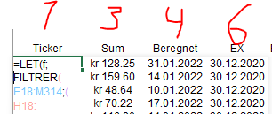
Index formula, can the column number be dynamic?

[Tirrazo]

I need help to set the column number for the index formula automatically instead of static.

The formula is used in combination with LET-function and the array that this creates are returning different values.
If I would like to increase the number of columns because I want more data within the area the formula is looking, I have to manually count the columns and enter it.
I have many if the same formulas so this takes a lot of time.

In the example I am using column 1,3,4,6 that I am getting data back from.

 

[awoohaw]

I can't understand your images. If you get the xl2bb add in https://www.mrexcel.com/board/mrexcel-xl2bb.svg you can help forum users help you better and more efficiently.
But regarding your question. The INDEX function has a secondary feature, it also returns the cell reference of the returned value. So, you can create a dynamic range like this:

Mr Excel Questions.xlsx
	A	B	C	D	E	F	G
3		Col A	Col B	Col C	Col D	Col E
4	1	263	189	219	124	200
5	2	254	120	173	102	294
6	3	219	195	123	297	150
7	4	276	222	163	128	130
8
9					Return:
10	Number of Values to return:			3	Col B
11	Column of Values to return:			Col B	189
12					120
13					195
14
Sheet8

Cell Formulas
Range	Formula
E10:E13	E10	=INDEX($B$3:$F$3,MATCH(D11,B3:F3,0)): INDEX($B$4:$F$7,MATCH($D$10,A4:A7,0), MATCH(D11,B3:F3,0))
Dynamic array formulas.

Cells with Data Validation
Cell	Allow	Criteria
D10	List	=$A$4:$A$7
D11	List	=$B$3:$F$3

 

[Tirrazo]

I can't understand your images. If you get the xl2bb add in https://www.mrexcel.com/board/mrexcel-xl2bb.svg you can help forum users help you better and more efficiently.
But regarding your question. The INDEX function has a secondary feature, it also returns the cell reference of the returned value. So, you can create a dynamic range like this:

Mr Excel Questions.xlsx
	A	B	C	D	E	F	G
3		Col A	Col B	Col C	Col D	Col E
4	1	263	189	219	124	200
5	2	254	120	173	102	294
6	3	219	195	123	297	150
7	4	276	222	163	128	130
8
9					Return:
10	Number of Values to return:			3	Col B
11	Column of Values to return:			Col B	189
12					120
13					195
14
Sheet8

Cell Formulas
Range	Formula
E10:E13	E10	=INDEX($B$3:$F$3,MATCH(D11,B3:F3,0)): INDEX($B$4:$F$7,MATCH($D$10,A4:A7,0), MATCH(D11,B3:F3,0))
Dynamic array formulas.

Cells with Data Validation
Cell	Allow	Criteria
D10	List	=$A$4:$A$7
D11	List	=$B$3:$F$3

Thank you!

I can try to install that add-in or can I upload a spreadsheet with my code so you can check it?
So what you actually say is that the Index function can look in a column which I have given a referance? So I can give each column a reference and no matter how I increase or remove columns, the Index will hold on to the column it was looking in from the start because of the reference I give it?

 

[awoohaw]

The index function provides two things. The first thing it does is used way more than the second... it returns a value according to the row and column criteria. The second thing it does is return the address REFERENCE of the the cell it finds. Were you able to copy my sheet snippet above and see how the formulas work?

In a table $E5:$G$7... you lookup INDEX($E$5:$E$7,2,2) you will get the value of cell F6. But if you use that formula in conjuction with a cell reference ... say $F$1 for example like this:
$F$1: INDEX($E$5:$E$7,2,2)
you will get a spilled array of the cells F1 thru F6. Even if you don't have an excel version that spills arrays, the array is still created, but you can only use aggregate functions on it. So you can do counts, SUMS, MINs, etc.

 

[awoohaw]

and putting that in a LET function makes it much more easier. So, if you are good with LET then you should be able to do this with ease.

 

[Tirrazo]

The index function provides two things. The first thing it does is used way more than the second... it returns a value according to the row and column criteria. The second thing it does is return the address REFERENCE of the the cell it finds. Were you able to copy my sheet snippet above and see how the formulas work?

In a table $E5:$G$7... you lookup INDEX($E$5:$E$7,2,2) you will get the value of cell F6. But if you use that formula in conjuction with a cell reference ... say $F$1 for example like this:
$F$1: INDEX($E$5:$E$7,2,2)
you will get a spilled array of the cells F1 thru F6. Even if you don't have an excel version that spills arrays, the array is still created, but you can only use aggregate functions on it. So you can do counts, SUMS, MINs, etc.

I haven't been able to do it yet, will try it out.
But would it be possible to name all my columns from column1 to column70 for example and tell the INDEX which column to return by a name (e.g column 45, column 50 and column 70)?

 

[awoohaw]

I'm not sure why you need that, but I don't fully understand your request so it could be important.
But the match function figures out your column to return already by reading the "column name" cell I created - which is text not a range of cells. You would have to update every INDEX statement with a hard coded column name (or use the INDIRECT statement in a different way to approach the task). When you try it ouit you may understand.

 

[Tirrazo]

I'm not sure why you need that, but I don't fully understand your request so it could be important.
But the match function figures out your column to return already by reading the "column name" cell I created - which is text not a range of cells. You would have to update every INDEX statement with a hard coded column name (or use the INDIRECT statement in a different way to approach the task). When you try it ouit you may understand.

Ok, I will try and see if I understand this a littlebit later and come back to you.
I can also make a workbook if I don't understand so you can see it.

 

[awoohaw]

Yes, that would be great. Look forward to more.

 

[Tirrazo]

Yes, that would be great. Look forward to more.

I have downloaded XL2BB and here is the mini sheet:

The add-in uses very long time, that's why there are so few cells.

Testark.xlsm
	G	H	I	J
350	IGM	kr 128.25	31.01.2022	30.12.2020
Utbk

Cell Formulas
Range	Formula
G350:J376	G350	=LET(f,FILTER(E18:M314,(H18:H314>=$DK$10)*(H18:H314<=$DK$11),""),IF(ISERR(ROWS(f))="","Ingen utbytte",SORT(INDEX(f,SEQUENCE(ROWS(f)),{1,3,4,6}),4)))
Dynamic array formulas.