Index > Match across broad (Column:Row) range

[sanantonio]

Hi All,

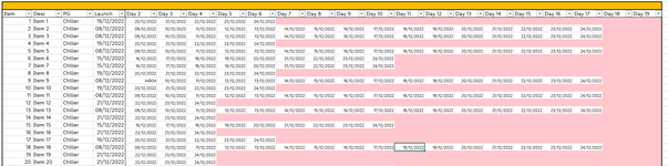
So I have a data set where items by day report back their sales, write offs etc. (Sheet1)

For reasons unsaid I need not the date of the sale but the day after launch. EG:

Item 1 was launched 26/12/2022, therefore in the picture above column S would say "Day 2".

I have the date of each "day after launch" in another worksheet: (Sheet2)

I have tried my trusty Index(Match) formula but it won't work. I'm presuming because of the range. My formula is in S4 on sheet1 thus:

=index(Sheet2!F3:U3,match(1,index((F4=Sheet2!B4:B999)*(H4=Sheet2!F4:U999),0,1),0))

Any ideas?

 

[KRice]

A simpler example to illustrate. Assume this on Sheet2:

Book4
	B	C	D	E	F	G	H	I	J
3					a	b	c	d	e
4	1				2	3	4	5	6
5	2				8	9	10	11	12
6	3				14	15	16	17	18
Sheet2

Then for Sheet1, the row index of interest first needs to be isolated:

MATCH($F4,Sheet2!$B$4:$B$999,0)

...so that the entire row necessary for the next comparison/matching can be identified...the row is isolated with this part of the formula (note the comma at the end, which is necessary):

INDEX(Sheet2!$F$4:$U$999,MATCH($F4,Sheet2!$B$4:$B$999,0),)

Then that isolated row is used to perform the date matching, although I'm not certain about this. My example uses an exact match with H4, but you might need a different type of match. I can't tell from the images you pasted. In any case, this matching step identifies the column index, which is then used to return the answer from F3:U3...

=INDEX(Sheet2!$F$3:$U$3,,MATCH($H4,INDEX(Sheet2!$F$4:$U$999,MATCH($F4,Sheet2!$B$4:$B$999,0),),0))

Book4
	F	G	H										R	S
4	1		5											d
Sheet1

Cell Formulas
Range	Formula
S4	S4	=INDEX(Sheet2!$F$3:$U$3,,MATCH($H4,INDEX(Sheet2!$F$4:$U$999,MATCH($F4,Sheet2!$B$4:$B$999,0),),0))

You could do this with some Excel 365 functions if desired, but post back about the date-matching issue I mentioned.

 

[sanantonio]

Hi. Thanks for responding.

I'm really sorry I'm totally lost with your explanation above. I must be doing something wrong as I can't get any of the formulas you posted to work, even though I've created an example that looks like yours.

Sheet2:

Sheet1:

 

[KRice]

Note that what I posted was roughly laid out similar to your original screenshots. The upper left cell in my posting of Sheet2 is B3, meaning that the a,b,c,d "headings" of interest are in row 3 with the numbers involved in matching found in rows 4 and down. I can't tell from your most recent posting whether you've done this. To avoid this type of issue, you might consider using the XL2BB add-in for exchanging small portions of your file. You should be able to copy my content directly by clicking on the small clipboard icon in the upper left of each snippet (which copies that snippet to your clipboard), then go to an empty worksheet, navigate to the same cell corresponding to the upper left of the snippet (B3 of Sheet2 for example) and paste. That places the content of the snippet and any formulas directly into your sheet.

 

[KRice]

From what I can guess, you have the Date of Sale in the Date column (col H) of Sheet1. Is that correct? And for Item 1 that date is shown as 27/12/2022 in cell H something...H3 maybe...I can't tell from the image.

You mentioned that Item 1 was launched 26/12/2022, but I don't see where that information comes from. I do not believe that is shown anywhere.

You want the "day after launch", which apparently is what Sheet2 shows. Yet Sheet2 shows a launch date (cell E4) of 19/12/2022 for Item 1...so I am confused. Was Item 1 "launched" on 26/12/2022 or 19/12/2022. If you want the "day after launch" could you simply add 1 to the date?

So I am not sure whether Sheet1 column H should be used at all. Assuming a date of interest appears on Sheet1 Column H (which I'll call the target date), I believe you want to find the smallest date that is larger than the target date and return the Day number associated with it. If that is true, then the exact match option is not correct, and none of the options readily available from match will work either, because they will find values that are either "exact or larger", or "exact or smaller". So these other options will still potentially find an exact match, which you do not want. Instead, you'll have to take a different approach. This is most easily done using some Excel 365 functions, although you can make it work with some additional logic in MATCH, and then you would need to find the minimum, etc.

After addressing these issues, then if a lookup is still needed (similar to the INDEX/MATCH shown earlier, except the min-greater-than-target condition needs to be applied), you could try something like this:

MrExcel_20231208.xlsx
	A	B	C	D	E	F	G	H	I	J	K	L	M
3						a	b	c	d	e	f	g
4		1				2	3	4	5	7	6	8
5		2				8	9	10	11	12	13	14
6		3				14	15	16	17	18	19	20
Sheet2

MrExcel_20231208.xlsx
	F	G	H										R	S
4	1		5											f
Sheet1

Cell Formulas
Range	Formula
S4	S4	=LET(itm,Sheet2!$B$4:$B$9,day,Sheet2!$F$3:$U$3,data,Sheet2!$F$4:$U$9,irow,FILTER(data,itm=$F4),a,FILTER(VSTACK(day,irow),irow>H4),TAKE(SORTBY(a,TAKE(a,-1)),1,1))

If you are unfamiliar with these functions, they essentially find the item row of interest and isolate it as the variable named irow. The day array in row 3 is called "day". We stack these two together vertically, and then filter them to show only the columns where the dates in irow are greater than the date in H4. Then we sort the result by the dates remaining and take the day associated with the smallest date.

 

[sanantonio]

Still rightly confused (I'm a simple soul) but the formula from your second post works a treat! Thank you very much

 

[KRice]

That’s good to hear…I’m happy to help.