Hi All,
I created a spreadsheet years ago in my previous job which did exactly what I want my new one too. However I have left the company now and dont have access to it to review the formula. Basically I have a sheet with =today() in cell AA1 (for example). I would like the following cells to list all the names (in col A) that have a number greater than 0 (in col B and later col C, D, E etc). I would like it to change based on the date which is listed at the top of the columns. Please see below for reference:
Data:
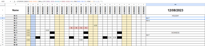
Dashboard:
Basically use AA1 as a reference to search B1:Z1. If finds the matching date, then search the column for anything over 0 and bring through the corresponding name in column A.
When the date changes in AA1 to 01/02/2023 for example, it would then reference the date and search column C1 etc.
Hope this makes sense? I have had a hiatus from formulas for about 2 years and had a blank and just cant get it right.
Thanks in advance
Dan
I created a spreadsheet years ago in my previous job which did exactly what I want my new one too. However I have left the company now and dont have access to it to review the formula. Basically I have a sheet with =today() in cell AA1 (for example). I would like the following cells to list all the names (in col A) that have a number greater than 0 (in col B and later col C, D, E etc). I would like it to change based on the date which is listed at the top of the columns. Please see below for reference:
Data:
| Name (A1) | 01/01/2023 (B1) | 01/02/2023 (C1) |
| Mr A (A2) | 5.00 | |
| Mr B (A3) | 5.00 | |
| Mr C | 0 | 2.75 |
| Mr D | 0 | 0 |
Dashboard:
| Date | 01/01/2023 (this is cell AA1 - list to change based on this cell) | |
| Holiday | ||
| Mr A (this is where I would want my list to start) | 5.00 (I would just use lookup to bring through the hours so this cell is fine, unless there is a formula for this too? im pretty sure I had one for each of the 8 columns in my last sheet that did this) | |
| Mr B |
|
Basically use AA1 as a reference to search B1:Z1. If finds the matching date, then search the column for anything over 0 and bring through the corresponding name in column A.
When the date changes in AA1 to 01/02/2023 for example, it would then reference the date and search column C1 etc.
Hope this makes sense? I have had a hiatus from formulas for about 2 years and had a blank and just cant get it right.
Thanks in advance
Dan
")


