Index/Match using two columns

[bjornc]

Hi guys,

i have this rather large data set that contains 80k rows.

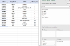
The first column is Supplier ID# number, the second column is our internal SKU# pn, and the last column is the MPN# (manufacturing pn). Each SKU# has multiple Suppliers, so you can assume that eg. SKU# 2468037is supplied by Supplier# 02580, X, Y... Z.

Supplier#	SKU#	MPN#
38756	9718122
02580	2468037	4031481
02147	2279467	EFAS-RF-16-400-450-17
03544	8602612	7683
01110	2035805
38756	9716736
03798	9821329	50810
03641	3000104
01110	2034315	700618925
10013	8605888	2600-040-900-000
12081	3257502	4317
03357	2511324	53406120
00742	2187962	22330

I need to make a list that looks something like this:

I have tried: "=INDEX($C$4:$C$61;MATCH($E5;$A$4:$A$61;0);MATCH(F$3;$B$4:$B$61;0))" with no success.

I managed to use an array formula which required me to use CTRL+SHIFT+ENTER, but i was not able to copy it into all the cells.

I am using Excel 2016. My computer is deeply locked into all kinds of secure stuff, i'm not able to install anything.

Thanks for the help in advance.

 

[steve the fish]

Before start if it has 80k rows why is your index only showing C4:C61?

 

[bjornc]

I copied the mere essentials because it was slowing down my computer. Here you can see the bottom of the original, i only need the first three columns.

 

[steve the fish]

I have a feeling you may be misunderstanding all this. How are you going to fill in all the supplier sku numbers and your sku numbers in the table you want? You will then get thousands of errors as you wouldnt ever expect a match unless every supplier supplies every sku.

 

[coban]

I have a feeling you may be misunderstanding all this. How are you going to fill in all the supplier sku numbers and your sku numbers in the table you want? You will then get thousands of errors as you wouldnt ever expect a match unless every supplier supplies every sku.

I know there will be missing data yes. But not to the extent you believe. If I can map each suppliers corresponding MPN to our SKU. Then I can map their price and place orders where they are the cheapest.

Is there a solution? I tried to wrangle the dataset into Pivot but was unable to return the MPN. Can this be done?

 

[AhoyNC]

Maybe something like this?
This is an array formula and must be entered with CTRL-SHIFT-ENTER.

Book1
	A	B	C	D	E	F	G	H	I	J	K	L	M	N	O
1	Supplier#	SKU#	MPN#
2	38756	9718122			Supplier#	38756	2580	2147	3544	1110	38756	3798	3641	1110	10013
3	2580	2468037	4031481		SKU# / MPN#
4	2147	2279467	EFAS-RF-16-400-450-17		9718122	0					0
5	3544	8602612	7683		2468037		4031481
6	1110	2035805			2279467			EFAS-RF-16-400-450-17
7	38756	9716736			8602612				7683
8	3798	9821329	50810		2035805					0				0
9	3641	3000104			9716736	0					0
10	1110	2034315	700618925		9821329							50810
11	10013	8605888	2600-040-900-000		3000104								0
12	12081	3257502	4317		2034315					700618925				700618925
13	3357	2511324	53406120		8605888										2600-040-900-000
14	742	2187962	22330		3257502
15					2511324
16					2187962
Sheet1

Cell Formulas
Range	Formula
F4:O16	F4	=IFERROR(INDEX($C$2:$C$14,MATCH(F$2&"/"&$E4,$A$2:$A$14&"/"&$B$2:$B$14,0)),"")

 

[steve the fish]

You could use a pivot table yes. Put the prices in the table and you could use it to see min prices based on sku. Put SKU#, Supplier# then MPN# in the rows and price in the values. Use 'min of' rather than sum.

 

[steve the fish]

And dont use a formula for this. Your computer may melt. There are 80k x 80k formulas required.

 

[steve the fish]

Heres one i made of your supplied data.

 

[bjornc]

Maybe something like this?
This is an array formula and must be entered with CTRL-SHIFT-ENTER.

Book1
	A	B	C	D	E	F	G	H	I	J	K	L	M	N	O
1	Supplier#	SKU#	MPN#
2	38756	9718122			Supplier#	38756	2580	2147	3544	1110	38756	3798	3641	1110	10013
3	2580	2468037	4031481		SKU# / MPN#
4	2147	2279467	EFAS-RF-16-400-450-17		9718122	0					0
5	3544	8602612	7683		2468037		4031481
6	1110	2035805			2279467			EFAS-RF-16-400-450-17
7	38756	9716736			8602612				7683
8	3798	9821329	50810		2035805					0				0
9	3641	3000104			9716736	0					0
10	1110	2034315	700618925		9821329							50810
11	10013	8605888	2600-040-900-000		3000104								0
12	12081	3257502	4317		2034315					700618925				700618925
13	3357	2511324	53406120		8605888										2600-040-900-000
14	742	2187962	22330		3257502
15					2511324
16					2187962
Sheet1

Cell Formulas
Range	Formula
F4:O16	F4	=IFERROR(INDEX($C$2:$C$14,MATCH(F$2&"/"&$E4,$A$2:$A$14&"/"&$B$2:$B$14,0)),"")

This is the solution i want. And it's the solution i managed to produce earlier, the main problem being that i was not able to copy the array formula down in any manner, so i had to copy paste each cell and then press CTRL+SHIFT+ENTER... How'd you manage to populate the matrix?