INDEX & MATCH with INDIRECT Function

IDRIS86

Board Regular
Joined
Mar 18, 2021
Messages
82
Office Version
  1. 365
Platform
  1. Windows
Hi I tried to match the argument in the below formula to -1 to pull the higher values than the look up value. But its not working. Only with Match argument 0 & 1 works. But I need to pick value higher than my reference. Could you assist.

Below the function,

=INDEX(INDIRECT(Table10[@MODEL]&"A"),MATCH(BC28,INDIRECT(Table10[@MODEL]&"H"),0),MATCH(BB28,INDIRECT(Table10[@MODEL]&"W"),0))
 

Excel Facts

Format cells as currency
Select range and press Ctrl+Shift+4 to format cells as currency. (Shift 4 is the $ sign).
You would need to provide an XL2BB version of Table10 and the values in BC28 & BB28 and your expected result.
On the face of it the use of Indirect doesn't seem to add any value.
 
Upvote 0
You would need to provide an XL2BB version of Table10 and the values in BC28 & BB28 and your expected result.
On the face of it the use of Indirect doesn't seem to add any value.
Hi Alex,
Thanks.
The table is made up a Dimensions called Width in column & Height in Row. If I enter lookup values let's say 329 in row & and 430 in Column. If this specific sizes are not in table, then I would need the corresponding values of next higher available sizes, let say 356 in Row and 457 in column.
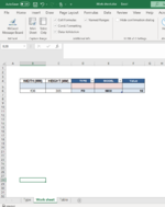
I dont know much formula to pick values for a referred size from a table located in other tabs. I referred this online & applied it. It works well & brought the required values. Only the concern is it doesnt go to next available higher sizes. I added both table 10 & the sheet where the values to be pulled. Kindly assist. Also I attached snapshot of my workbook how it looks.

Table 10

Work sheet.xlsx
EFGHIJKLMNOPQRSTU
10SIZE1021522032543053564064575085596106602900295030003048
11102535962666972758285899298420420420420
12152565962667275798285929598433433433433
1320359626672757985899298102105459459459459
1425459666972758285899598105108473473473473
153056269727982899295102108112115512512512512
1635666727582859295102108112118125538538538538
17406697579859295102108112118125131564564564564
184577279859295102108115118128131138604604604604
1950875828995102108115121128135141148643643643643
2055979859298105112118125131141148154669669669669
21610828995102108115121128135144151158683683683683
22660859298105112121128135141151158164722722722722
237118995102112118125135141148158164174761761761761
247629298105115121131138148154164171180788788788788
2581395102112118128135144151161171180187827827827827
2686495105115121131141148158167177187194853853853853
2791498108118128135144154164174184194200879879879879
289501511641771902032172302432562692822951286128612861286
2910001511641771902032172302432562692822951286128612861286
3010501581711841972102232362492632822953081339133913391339
3111001581711841972102232362492632822953081339133913391339
3211501641771902032172302432562692893023151365136513651365
3312001641771902032172302432562692893023151365136513651365
3412501711841972102232432562692823023153281444144414441444
3513001711841972102232432562692823023153281444144414441444
3613501771902032232362492692822953153283481523152315231523
3714001771902032232362492692822953153283481523152315231523
3814501841972102302432632762953083283413611575157515751575
3915001841972102302432632762953083283413611575157515751575
4015501902032232362562692893023223413613741654165416541654
4116001902032232362562692893023223413613741654165416541654
4216501902102302432632822953153353543743871706170617061706
4317001902102302432632822953153353543743871706170617061706
4417501972172362562692893083283483683874001759175917591759
4518001972172362562692893083283483683874001759175917591759
4618292462662853053253453643844044334534732048204820482048
Table
Cells with Conditional Formatting
CellConditionCell FormatStop If True
F11:U46Cell Value=0textNO


Other sheet in same in work book with the required input conditions,

Work sheet.xlsx
BCDEF
4WIDTH (MM)HEIGHT (MM)TYPEMODELValue
5
6457254 FD IBD2 89
Work sheet
Cell Formulas
RangeFormula
F6F6=INDEX(INDIRECT(Table10[@MODEL]&"A"),MATCH(C6,INDIRECT(Table10[@MODEL]&"H"),0),MATCH(B6,INDIRECT(Table10[@MODEL]&"W"),0))
Cells with Conditional Formatting
CellConditionCell FormatStop If True
D6Cell Value=0textNO
E6Cell Value=0textNO
D6Cell Value=0textNO
E6Cell Value=0textNO
D5Cell Value=0textNO
E5Cell Value=0textNO
D5Cell Value=0textNO
E5Cell Value=0textNO
F6Cell Value=0textNO
Cells with Data Validation
CellAllowCriteria
D5:D6List=TYPE
E5:E6List=INDIRECT(D5)


You would need to provide an XL2BB version of Table10 and the values in BC28 & BB28 and your expected result.
On the face of it the use of Indirect doesn't seem to add any value.
 

Attachments

  • Work book.PNG
    Work book.PNG
    43.1 KB · Views: 7
Upvote 0
How about
+Fluff 1.xlsm
ABCDEF
1
2
3
4WIDTH (MM)HEIGHT (MM)TYPEMODELValue
5
6450250 FD IBD2 89
Test
Cell Formulas
RangeFormula
F6F6=INDEX(Table!$F$11:$U$46,XMATCH(C6,Table!E11:E46,1),XMATCH(B6,Table!F10:U10,1))
 
Upvote 0
How about
+Fluff 1.xlsm
ABCDEF
1
2
3
4WIDTH (MM)HEIGHT (MM)TYPEMODELValue
5
6450250 FD IBD2 89
Test
Cell Formulas
RangeFormula
F6F6=INDEX(Table!$F$11:$U$46,XMATCH(C6,Table!E11:E46,1),XMATCH(B6,Table!F10:U10,1))
Thanks. But Will this formula refer to the respective table by its name. Because I will have multiple tables at table sheet. Upon giving input such as Width , height & model, it needs to look at the respective table of that model and revert the values.
 
Upvote 0
No it will look at the specific range in the formula, because you gave no other information.
 
Upvote 0
No it will look at the specific range in the formula, because you gave no other information.
I just replaced MATCH function with your XMATCH function with Match 1 in my existing formula. It takes higher value as what I needed. It looks working.

=INDEX(INDIRECT(Table10[@MODEL]&"A"),XMATCH(D28,INDIRECT(Table10[@MODEL]&"H"),1 ),XMATCH(C28,INDIRECT(Table10[@MODEL]&"W"),1 ))
 
Upvote 0
Glad you sorted it & thanks for the feedback.
 
Upvote 0
Hi, Can you advise. The formula works. But if I copy the whole row and paste next line item. I couldnt find the issue. Could you advise.

Work sheet.xlsx
BCDEF
4WIDTH (MM)HEIGHT (MM)TYPEMODELValue
5
6530508 FD IBD2 135
7530508 FD IBD2 #VALUE!
Work sheet
Cell Formulas
RangeFormula
F6:F7F6=INDEX(INDIRECT(Table10[@MODEL]&"A"),XMATCH(C6,INDIRECT(Table10[@MODEL]&"H"),1),XMATCH(B6,INDIRECT(Table10[@MODEL]&"W"),1))
Cells with Conditional Formatting
CellConditionCell FormatStop If True
D7Cell Value=0textNO
E7Cell Value=0textNO
D7Cell Value=0textNO
E7Cell Value=0textNO
F7Cell Value=0textNO
D6Cell Value=0textNO
E6Cell Value=0textNO
D6Cell Value=0textNO
E6Cell Value=0textNO
D5Cell Value=0textNO
E5Cell Value=0textNO
D5Cell Value=0textNO
E5Cell Value=0textNO
F6Cell Value=0textNO
Cells with Data Validation
CellAllowCriteria
D5:D7List=TYPE
E5:E7List=INDIRECT(D5)
 
Upvote 0

Forum statistics

Threads
1,215,214
Messages
6,123,664
Members
449,114
Latest member
aides

We've detected that you are using an adblocker.

We have a great community of people providing Excel help here, but the hosting costs are enormous. You can help keep this site running by allowing ads on MrExcel.com.
Allow Ads at MrExcel

Which adblocker are you using?

Disable AdBlock

Follow these easy steps to disable AdBlock

1)Click on the icon in the browser’s toolbar.
2)Click on the icon in the browser’s toolbar.
2)Click on the "Pause on this site" option.
Go back

Disable AdBlock Plus

Follow these easy steps to disable AdBlock Plus

1)Click on the icon in the browser’s toolbar.
2)Click on the toggle to disable it for "mrexcel.com".
Go back

Disable uBlock Origin

Follow these easy steps to disable uBlock Origin

1)Click on the icon in the browser’s toolbar.
2)Click on the "Power" button.
3)Click on the "Refresh" button.
Go back

Disable uBlock

Follow these easy steps to disable uBlock

1)Click on the icon in the browser’s toolbar.
2)Click on the "Power" button.
3)Click on the "Refresh" button.
Go back
Back
Top