Intuitively I'd expected to combine FILTER, SORT and UNIQUE but I can't get them to do what I want.

[IfAllElseFails]

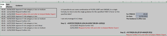
I want a SINGLE formula to return a SINGLE value from a table:
1) matching, in one column, a specified item
2) also, matching, in a second column, the highest date which is lower than a specified date

I can only manage it in 2 steps

I'm still getting to grips with functions which return multiple results

Help much appreciated
(sorry can't use the addin to upload a mini sheet - locked down corporate excel install)

 

[dreid1011]

Maybe this:

Book1
	A	B	C	D	E	F	G	H	I	J
1	Item ID	Date Effective	Guidance
2	45.02	9/23/2023	Approve if risk category is low or medium
3	45.02	12/12/2022	Request further info
4	45.02	1/11/2023	Request further info and refer to Subject Matter Expert						For Item ID	45.02
5	45.02	7/14/2023	Approve if risk category is low						On Date	3/15/2023
6	65.01	9/23/2023	Approve if risk category is low or medium						The Guidance in effect was
7	65.01	1/11/2023	Request further info
8	65.01	7/14/2023	Approve if risk category is low						1/11/2023	Request further info and refer to Subject Matter Expert
9	65.01	1/1/2024	Approve if risk category is not critical
10	19.12	9/23/2023	Approve if risk category is low or medium
11	19.12	1/11/2023	Request further info
Sheet2

Cell Formulas
Range	Formula
I8:J8	I8	=CHOOSEROWS(SORT(FILTER(B:C,((A:A=J4)*(B:B<=J5))),1,-1),1)
Dynamic array formulas.

 

[felixstraube]

How about?:

Book1
	A	B	C	D	E	F	G	H	I	J
1	Item ID	Date Effective	Guidance
2	45.02	23/09/2023	A						Item ID	45.02
3	45.02	12/12/2023	B						On Date	15/03/2023
4	45.02	10/01/2023	THIS
5	45.02	14/07/2023	D						Result	THIS
6	65.01	23/09/2023	AA
7	65.01	12/12/2023	BB
8	65.01	10/01/2023	CC
9	65.01	14/07/2023	DD
Sheet2

Cell Formulas
Range	Formula
J5	J5	=FILTER(C:C,(A:A=$J$2)*(B:B=MAX(IFERROR(B:B*(B:B<=$J$3)*(A:A=$J$2),0))))

 

[Fluff]

Hi & welcome to MrExcel.
How about

=TAKE(SORT(FILTER(B2:B1000,(A2:A1000=J4)*(B2:B1000<=J5)),1,-1),1,-1)

It's always best to avoid using whole column references in array formulae.

 

[JamesCanale]

MrExcelPlayground20 (version 1).xlsb
	A	B	C	D	E
1	Item	Date	Guidance
2	45.02	9/23/2023	Thing1	Item	45.02
3	45.02	12/12/2022	Thing2	Date	3/23/2023
4	45.02	1/11/2023	Thing3
5	45.02	7/14/2023	Thing4		Thing3
6	65.01	9/23/2023	Thing5
7	65.01	1/11/2023	Thing6
8	65.01	7/14/2023	Thing7
9	65.01	1/1/2024	Thing8
10	19.12	9/23/2023	Thing9
11	19.12	1/11/2023	Thing10
Sheet24

Cell Formulas
Range	Formula
E5	E5	=INDEX(CHOOSECOLS(SORT(FILTER(B2:C11,A2:A11=E2),1),2),MATCH(E3,CHOOSECOLS(SORT(FILTER(B2:C11,A2:A11=E2),1),1),1))

 

[IfAllElseFails]

Thanks, that nearly worked - it returns both the date and the guidance.
But following your example and wrapping it with CHOOSECOLS does the trick!

 

[dreid1011]

Thanks, that nearly worked - it returns both the date and the guidance.
But following your example and wrapping it with CHOOSECOLS does the trick!

In that case, you should use Fluff's suggestion in post #4. The TAKE does the same as both CHOOSEROWS and CHOOSECOLS combined.

 

[felixstraube]

I thought you wanted only the text in column C. Formula in post 3 does that.

 

[felixstraube]

Taking @Fluff 's suggestion into account, not to use whole columns:

Book1
	A	B	C	D	E	F	G	H	I	J
1	Item ID	Date Effective	Guidance
2	45.02	23/09/2023	A						Item ID	45.02
3	45.02	12/12/2023	B						On Date	15/03/2023
4	45.02	10/01/2023	THIS
5	45.02	14/07/2023	D						Result	THIS
6	65.01	23/09/2023	AA
7	65.01	12/12/2023	BB
8	65.01	10/01/2023	CC
9	65.01	14/07/2023	DD
Sheet2

Cell Formulas
Range	Formula
J5	J5	=FILTER(C1:C1000,(A1:A1000=$J$2)*(B1:B1000=MAX(IFERROR(B1:B1000*(B1:B1000<=$J$3)*(A1:A1000=$J$2),0))))

 

[Fluff]

I thought you wanted only the text in column C. Formula in post 3 does that.

So do the formulae in post#4 & 5