Want2BExcel
Board Regular
- Joined
- Nov 24, 2021
- Messages
- 112
- Office Version
- 2016
- Platform
- Windows
Is it possible to make a button that changes the formula?
Right now the formula is "pointing" to the expected.expenses. but when a month is over I import all the actual expenses in a new sheet. Now I, of course, know what I have to do to change the formula to point to the new sheet. But if I gave this budget to friends, they don't know what to do. So if there was a button, they just could click on and then a drop-down menu opens to choose witch month he/she would like to apply the "new" formula...voila")
So from this:
Original in danish: =SUM.HVIS(ANSLÅET.UDGIFTER[Tekst];[@[Postering tekst]];ANSLÅET.UDGIFTER[Januar])
In english: =SUMIF(EXPECTED.EXPENSES[Text];[@[Postering text]];EXPECTED.EXPENSES[January])
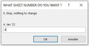
The user pushes the button and a dropdown menu opens with all 12 months to choose from. Pick January and the formulas in all rows in that whole column (January) changes to...
To this:
Original in danish: =SUM.HVIS(BUDGET_JAN_22[Tekst];[@[Postering tekst]];BUDGET_JAN_22[Beløb])
In english: =SUMIF(BUDGET_JAN_22[Text];[@[Postering text]];BUDGET_JAN_22[Amount])
It would be amazing!
Right now the formula is "pointing" to the expected.expenses. but when a month is over I import all the actual expenses in a new sheet. Now I, of course, know what I have to do to change the formula to point to the new sheet. But if I gave this budget to friends, they don't know what to do. So if there was a button, they just could click on and then a drop-down menu opens to choose witch month he/she would like to apply the "new" formula...voila
So from this:
Original in danish: =SUM.HVIS(ANSLÅET.UDGIFTER[Tekst];[@[Postering tekst]];ANSLÅET.UDGIFTER[Januar])
In english: =SUMIF(EXPECTED.EXPENSES[Text];[@[Postering text]];EXPECTED.EXPENSES[January])
The user pushes the button and a dropdown menu opens with all 12 months to choose from. Pick January and the formulas in all rows in that whole column (January) changes to...
To this:
Original in danish: =SUM.HVIS(BUDGET_JAN_22[Tekst];[@[Postering tekst]];BUDGET_JAN_22[Beløb])
In english: =SUMIF(BUDGET_JAN_22[Text];[@[Postering text]];BUDGET_JAN_22[Amount])
It would be amazing!