List unique values and count cell values with different conditions

[nahaku]

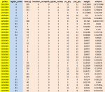
Hello, I im trying to find formulas to help me make statistics, but I do not know how to get this. The formulas I found on internet helps always only with half of the problem.
I am trying to list unique value from [A] Yelow column for example GBL0004,GBS0083,...
then it could list GBL0004 divided by Region name from Column Blue column so for example GBL0004 A , GBS0083 A, GBS0083 C1, GBS0083 B1,GBS0088 A, GBS0088 B1 ....
it basically splits the person by location where they ware working.
and then just count with Brown Columns separetly. That is somethink i might do, but I am not able to count it with that condition so it would count for unique
IF (Picker [A]+ Region name ) = SUM(C:C) { or Sum D, E, F, G......}

 

[nahaku]

Try
=UNIQUE(FILTER(FILTER(PSdata!$B$2:$E$508,(COLUMN(PSdata!$B2:$E2)=2)+(COLUMN(PSdata!$B2:$E2)=5)),NOT(ISERROR(MATCH(PSdata!B2:B508,L2:L20,0))))

Worked like charm :P
Hopefully last thing with all this listing of values.
I do not need the 2. cell list. Only list all unique GBS from cell "D" if they are unique and they are in my list of approved names from "AM6:AM24"
=UNIQUE(FILTER(PackData!D2:D15000,(COLUMN(PackData!$D2:$D2)=4)),NOT(ISERROR(MATCH(PackData!D2:D15000,AM6:AM24,0))))
I think it is working, but because of the "D2:D15000" range it is showing so many 0, is it possible to not show 0, ignore them in the list?

 

[Fluff]

How about
=UNIQUE(FILTER(PackData!D2:D15000,(PackData!$D2:$D15000<>"")*(NOT(ISERROR(MATCH(PackData!D2:D15000,AM6:AM24,0))))))

 

[nahaku]

How about
=UNIQUE(FILTER(PackData!D2:D15000,(PackData!$D2:$D15000<>"")*(NOT(ISERROR(MATCH(PackData!D2:D15000,AM6:AM24,0))))))

Exactly :P, Ok, I wish you nice Easter. I will try to not to bother at least until it is finished. Bless you.

 

[Fluff]

You're welcome & thanks for the feedback

 

[nahaku]

You're welcome & thanks for the feedback

Heh, Sorry, every day I get some new task it seems, no matter if there is world situation or not. I manage to get it done basically but i found one problem with my excel.
In my list is list of items what needs to be scanned with their current location. But i found out there are items in list with multiple entries and their locations. Is possible to make something so when I insert the barcode in the cell "C19" it will show entries for all same items? only difference should be in Quantity and Location I think. so if it could show them next to it?or maybe even under somehow, i have about 1000 entries in Refference table.

Scanning Test.xlsx
	A	B	C	D	E	F	G	H	I	J	K	L
1	Refference Table
2	No.	SKU	UPC	Name	QTY	Location	Status
3	1	1asd65sa1d	xxx	auto	1	001.09.3.1	Not Seen
4	2	65asd65	zzzxxcvnm	mobil	1	001.09.3.1	Scanned
5	3	1zxc6zxc6	adsda	motorka	2	001.22.1.1	Not Seen
6	4	3zxcsad6	zxczv	slnko	1	001.25.3.1	Scanned
7	5	4zxc9xz4c	zxvgag	babika	1	001.32.1.1	Not Seen
8	6	6z4xc6zx4c	asdzxv	sito	1	999.90.1.1	Not Seen
9	7	5xzc6z4xc6	hgfhjfg	kvety	1	999.90.1.1	Not Seen
10	8	65zxc654xcz	dsvxc	kozi	1	999.90.1.1	Not Seen
11	9	2xcz64zxc6	asdfzxc	lodka	1	999.90.1.1	Scanned
12	10	f64sdf6	asfxzc	pulover	4	999.90.1.1	Not Seen
13	11	gfd64g	safzxvc	slimak	1	999.90.1.1	Not Seen
14	12	3zxcsad6	haf	slnko	1	999.90.1.1	Scanned
15	13	3v5zxv8sa	ncvbcv	parkovisko	2	999.90.1.1	Not Seen
16
17			"C" Cells	items what were scanned and check against the Refference Table
18		18	Scanned SKU Barcode	Name	QTY	Location	QTY	Location	QTY	Location	QTY	Location
19		19	65asd65	mobil	1	001.09.3.1
20		20	3zxcsad6	slnko	1	001.25.3.1
21		21	2xcz64zxc6	lodka	1	999.90.1.1
22		22		Not Found
23		23		Not Found
24		24		Not Found
Sheet2

Cell Formulas
Range	Formula
G3:G15	G3	=IF(OR(COUNTIF($C$19:$C$35,"*"&$B$3:$B$15&"*")),"Scanned", "Not Seen")
D22:D24,D19:F21	D19	=IFERROR(XLOOKUP($C19,$B$3:$B$15,$D$3:$F$15,"Not Found",0,1),"")
Dynamic array formulas.

 

[nahaku]

I tried to use =IFERROR(INDEX($B$3:$G$15, SMALL(IF("$C19"=$B$3:$B$15, ROW($F$3:$F$15)-2,"TEST1"), COLUMN()-5)),"TEST2") but it always shows only the error=TEST2 in cell... It does not check the C19 against the B3:B15 range, but when i checked the function it was showing True for the B4 Column .... I dont know

 

[Fluff]

As this is a totally different question, you will need to start a new thread. Thanks