List unique values and count cell values with different conditions

[nahaku]

Hello, I im trying to find formulas to help me make statistics, but I do not know how to get this. The formulas I found on internet helps always only with half of the problem.
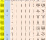
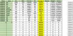
I am trying to list unique value from [A] Yelow column for example GBL0004,GBS0083,...
then it could list GBL0004 divided by Region name from Column Blue column so for example GBL0004 A , GBS0083 A, GBS0083 C1, GBS0083 B1,GBS0088 A, GBS0088 B1 ....
it basically splits the person by location where they ware working.
and then just count with Brown Columns separetly. That is somethink i might do, but I am not able to count it with that condition so it would count for unique
IF (Picker [A]+ Region name ) = SUM(C:C) { or Sum D, E, F, G......}

 

[Fluff]

You could use a list like

+Fluff.xlsm
	A	B	C	D	E	F	G	H	I
1	County		Ward
2	Cumbria		A		Cheshire		Derbyshire	A
3	Derbyshire		A		Cumbria		West Yorkshire	B
4	Derbyshire		A		Somerset		Derbyshire	B
5	West Yorkshire		B				West Yorkshire	C
6	Derbyshire		B				Derbyshire	C
7	Derbyshire		B				Staffordshire	C
8	West Yorkshire		C				Derbyshire	D
9	Derbyshire		C				West Yorkshire	E
10	Staffordshire		C				Greater Manchester	E
11	Derbyshire		D				West Yorkshire	F
12	Derbyshire		D				Staffordshire	A
13	Cheshire		D				Shropshire	B
14	West Yorkshire		E				County Durham	B
15	Greater Manchester		E				Lancashire	C
16	West Yorkshire		E				Northumberland	D
17	West Yorkshire		F				Lancashire	D
18	West Yorkshire		F				South Yorkshire	D
19	West Yorkshire		F				Derbyshire	E
20	Staffordshire		A				County Durham	F
21	Somerset		A
22	Cumbria		A
Data

Cell Formulas
Range	Formula
G2:H20	G2	=UNIQUE(FILTER(FILTER(A2:C37,(COLUMN(A2:C2)=1)+(COLUMN(A2:C2)=3)),ISERROR(MATCH(A2:A37,E2:E4,0))))
Dynamic array formulas.

 

[nahaku]

AMAZING <3 Thank you.
All the best.

 

[Fluff]

You're welcome & thanks for the feedback

 

[nahaku]

I tried to use your function, but instead of ignoring the Values from the Table on side, I would want to use this time only those values. It is kind a working but for some reason when i added data from different date, it was showing also values for GBS0203 , even when it is not in my list, and all other values what I do not want in my Tab are ignored... Weird.

End of day report.xlsx
	A	B	C	D	E	F	G	H	I	J	K	L
1	Picker	Zone	Ocs	SKUs	Time	Pcs	Avarage T	Repicks	Weight	Volume
2	GBS0183	D3	12965	1024	7604476	32854	231.46	0	3.5014	12.309987		GBS0166
3	GBS0183	D2	268	43	265053	430	616.40	0	0.12175	0.5224799		GBS0183
4	GBS0183	LE	341	157	284507	525	541.92	0	0.09364	0.3961211		GBS0184
5	GBS0183	D3,D2	375	173	224833	725	310.11	0	0.20202	1.0498044		GBS0184
6	GBS0183	D2,LE,D3	70	32	180810	97	1864.02	0	0.03339	0.1245715		GBS0185
7	GBS0183	D2,D3	193	50	207628	734	282.87	0	0.04116	0.1837786		GBS0190
8	GBS0183	LE,D3	985	10	42797	4874	8.78	0	0.13361	0.2139432		GBS0192
9	GBS0183	D3,LE	72	12	11939	92	129.77	0	0.01233	0.0226128		GBS0196
10	GBS0203	C1	284	7	4783	284	16.84	3	3.0125	27.624641		GBS0218
11	GBS0203	B1	10	1	992	10	99.20	0	0.175	1.52134		GBS0219
12	GBS0203	B2	50	1	549	50	10.98	0	0.915	3.4056		GBS0221
13	0	0	0	0	0	0	#DIV/0!	0	0	0		GBS0225
14			0	0	0	0	#DIV/0!	0	0	0		GBS0226
15			0	0	0	0	#DIV/0!	0	0	0		GBS0227
16			0	0	0	0	#DIV/0!	0	0	0		GBS0228
17			0	0	0	0	#DIV/0!	0	0	0		GBS0229
18			0	0	0	0	#DIV/0!	0	0	0		GBS0230
19			0	0	0	0	#DIV/0!	0	0	0		GBS0234
20			0	0	0	0	#DIV/0!	0	0	0		GBS0235
Picker Stat.

Cell Formulas
Range	Formula
A2:B13	A2	=UNIQUE(FILTER(FILTER(PSdata!$B$2:$E$508,(COLUMN(PSdata!$B2:$E2)=2)+(COLUMN(PSdata!$B2:$E2)=5)),ISERROR(MATCH(PSdata!B2:B508,L2:L20,-1))))
C2:C20	C2	=SUMIFS(PSdata!O:O,PSdata!$B:$B,$A2,PSdata!$E:$E,$B2)
D2:D20,F2:F20	D2	=SUMIFS(PSdata!N:N,PSdata!$B:$B,$A2,PSdata!$E:$E,$B2)
E2:E20	E2	=SUMIFS(PSdata!K:K,PSdata!$B:$B,$A2,PSdata!$E:$E,$B2)
G2:G20	G2	=E2/F2
H2:H20	H2	=SUMIFS(PSdata!M:M,PSdata!$B:$B,$A2,PSdata!$E:$E,$B2)
I2:J20	I2	=SUMIFS(PSdata!Q:Q,PSdata!$B:$B,$A2,PSdata!$E:$E,$B2)
Dynamic array formulas.

Cells with Conditional Formatting
Cell	Condition		Cell Format	Stop If True
L2:L20	Cell Value	duplicates	text	NO
L2:L20	Cell Value	duplicates	text	NO
L2:L20	Cell Value	duplicates	text	NO
L2:L20	Cell Value	duplicates	text	NO

 

[nahaku]

I followed the guide how to import it but it does not work...
I tried to use your function, but instead of ignoring the Values from the Table on side, I would want to use this time only those values. It is kind a working but for some reason when i added data from different date, it was showing also values for GBS0203 , even when it is not in my list, and all other values what I do not want in my Tab are ignored... Weird.

=UNIQUE(FILTER(FILTER(PSdata!$B$2:$E$508,(COLUMN(PSdata!$B2:$E2)=2)+(COLUMN(PSdata!$B2:$E2)=5)),ISERROR(MATCH(PSdata!B2:B508,L2:L20,-1))))

I tried XMATCH with 0 , but then I got No output...

 

[Peter_SSs]

I followed the guide how to import it but it does not work...

After pasting the XL2BB code in your reply, I think you had (accidentally?) selected some of the code and clicked the strikethrough icon above the Reply window

I have fixed it for you.

 

[nahaku]

heh do not know how that happend, I tried it like 10 times with preview, and it was every single time. So i thought preview was broken :P

 

[Peter_SSs]

heh do not know how that happend, I tried it like 10 times with preview, and it was every single time. So i thought preview was broken :P

Suggest that you go to the Test Here forum and have a practice or two to see if you can get XL2BB working.

 

[nahaku]

You're welcome & thanks for the feedback

Sorry to bother again, I tried to adjust the formula for another purpose, and when i use
=UNIQUE(FILTER(FILTER(PSdata!$B$2:$E$508,(COLUMN(PSdata!$B2:$E2)=2)+(COLUMN(PSdata!$B2:$E2)=5)),ISERROR(MATCH(PSdata!B2:B508,AG5:AG24,-1))))
It will list only GBS names what are in the list on Right side in post number #14. But for some reason it still Shows in Tab GBS0203, even when it is not in my list.
To me it looks like it is showing values close to values of my list. I tried to use XMATCH function instead of MATCH but either it was same result or I got error. Do you have any advice?
I now need just to extract names what are in the DATA if they are in my list on the right side of post #14 :{

 

[Fluff]

Try
=UNIQUE(FILTER(FILTER(PSdata!$B$2:$E$508,(COLUMN(PSdata!$B2:$E2)=2)+(COLUMN(PSdata!$B2:$E2)=5)),NOT(ISERROR(MATCH(PSdata!B2:B508,L2:L20,0))))