Look up 2 conditions in 2 sheets

[colzre]

Hello experts,

I am trying to look up 2 conditions in 2 different sheets.

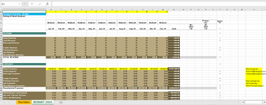
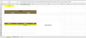
Formula is in cell D13 on "Numbers" sheet to get 1st condition based on F13 and look for it on sheet "BUDGET 2024" cells X30:X37. 2nd condition based on "Numbers" sheet cell B1 and look for it on sheet "BUDGET2024" cells B1:M1.

Then return the data from the table on "BUDGET 2024" sheet cells B17:M42 when both conditions are met.

This would return the amount of 228,836.54 which sits on "BUDGET 2024" cell B30 however I get an error.

All cells in questions are highlighted in yellow background.


Any help would be highly appreciated.


Thanks,

John

 

[awoohaw]

What is your formula and what is your error? Also, you say row 30, which has "Room Expenses" but then ask about "Room Revenue".

It would be HUGE help if you'd use the xl2bb add in (Link Below) and post a mini worksheet of your data. Posting images means the forum needs to recreate your data. And your data is all over the page and the forum could have typos and other error that can lead to confusion by you and the forum. If you cannot use the add in, then post your data as a table please, but tell us the top right cell address of the table so we can build the formula with matching cell references.

Thanks in advance.

 

[colzre]

Thank you for your response.

I have amended Room Revenue for Room expenses as meant to be. Apologies. See the Mini Sheets please.

file.xlsx
	A	B	C	D	E	F
1		1
2
3
4		Jan-24
5		Current		Budget
6
7
8
9
10
11
12		Actual	%	Budget	%
13				#VALUE!		Room expenses
Numbers

Cell Formulas
Range	Formula
D13	D13	=+XLOOKUP(F13,'BUDGET 2024'!X30:X39,XLOOKUP(Numbers!B1,'BUDGET 2024'!B1:M1,'BUDGET 2024'!B7:M86))

Cells with Data Validation
Cell	Allow	Criteria
B4:E4	List	=$BP$1:$BP$12

file.xlsx
	A	B	C	D	E	F	G	H	I	J	K	L	M	N	O	P	Q	R	S	T	U	V	W	X
1		1	2	3	4	5	6	7	8	9	10	11	12
2	Statement of Income - Budget
3	Rolling 12 Month Budcast
4	20/01/2024
5		Budcast	Budcast	Budcast	Budcast	Budcast	Budcast	Budcast	Budcast	Budcast	Budcast	Budcast	Budcast					Projection		HideFilter
6		Jan-24	Feb-24	Mar-24	Apr-24	May-24	Jun-24	Jul-24	Aug-24	Sep-24	Oct-24	Nov-24	Dec-24	Total		dic 2023 T12		dic 2022 T12		1
7	Statement of Income
8	Rooms Available	20	20	20	20	20	20	20	20	20	20	20	20	240.00						1
9	Rooms Sold	20	20	20	20	20	20	20	20	20	20	20	20	240.00						1
10	ADR	20	20	20	20	20	20	20	20	20	20	20	20	240.00						1
11	Occupancy%	20	20	20	20	20	20	20	20	20	20	20	20	240.00						1
12	RevPAR	20	20	20	20	20	20	20	20	20	20	20	20	240.00						1
13	Total RevPAR	20	20	20	20	20	20	20	20	20	20	20	20	240.00						1
14
15	REVENUE																			1
16
17	Room Revenue	20	20	20	20	20	20	20	20	20	20	20	20	240.00						1
18	Food Revenue	20	20	20	20	20	20	20	20	20	20	20	20	240.00						0
19	Beverage Revenue	20	20	20	20	20	20	20	20	20	20	20	20	240.00
20	Beach Club Revenue (Only for GHI)	20	20	20	20	20	20	20	20	20	20	20	20	240.00
21	Events Revenue	20	20	20	20	20	20	20	20	20	20	20	20	240.00						0
22	Parking Revenue	20	20	20	20	20	20	20	20	20	20	20	20	240.00						0
23	Spa Revenue	20	20	20	20	20	20	20	20	20	20	20	20	240.00
24	Miscellaneous Revenue	20	20	20	20	20	20	20	20	20	20	20	20	240.00
25	TOTAL REVENUE	160.00	160.00	160.00	160.00	160.00	160.00	160.00	160.00	160.00	160.00	160.00	160.00	1,920.00						1
26
27
28	EXPENSES																			1
29
30	Room Expenses	228,836.54	189,465.30	316,821.67	428,821.00	524,121.00	535,665.00	444,665.00	402,421.40	522,421.00	449,821.00	242,621.00	226,665.00	4,512,344.91										Room Expenses
31	Food Expenses	20.00	20.00	20.00	20.00	20.00	20.00	20.00	20.00	20.00	20.00	20.00	20.00	240.00						1				Food and Beverage Expenses
32	Beverage Expenses	20.00	20.00	20.00	20.00	20.00	20.00	20.00	20.00	20.00	20.00	20.00	20.00	240.00						0				Food and Beverage Expenses
33	Beach Club Expenses (Only for GHI)	20.00	20.00	20.00	20.00	20.00	20.00	20.00	20.00	20.00	20.00	20.00	20.00	240.00
34	Events Expenses	20.00	20.00	20.00	20.00	20.00	20.00	20.00	20.00	20.00	20.00	20.00	20.00	240.00						0
35	Parking Expenses	20.00	20.00	20.00	20.00	20.00	20.00	20.00	20.00	20.00	20.00	20.00	20.00	240.00						0				Parking Expenses
36	Spa Expenses	20.00	20.00	20.00	20.00	20.00	20.00	20.00	20.00	20.00	20.00	20.00	20.00	240.00										SPA Expenses
37	Miscellaneous Expenses	20.00	20.00	20.00	20.00	20.00	20.00	20.00	20.00	20.00	20.00	20.00	20.00	240.00						0				Other Income Expenses
38	Departmental Expenses	228,976.54	189,605.30	316,961.67	428,961.00	524,261.00	535,805.00	444,805.00	402,561.40	522,561.00	449,961.00	242,761.00	226,805.00	4,514,024.91						1
39
40	Administrative and General	20.00	20.00	20.00	20.00	20.00	20.00	20.00	20.00	20.00	20.00	20.00	20.00	513,068.92						1
41	Info and Telecom Systems	20.00	20.00	20.00	20.00	20.00	20.00	20.00	20.00	20.00	20.00	20.00	20.00	29,403.10						1
42	Sales and Marketing	20.00	20.00	20.00	20.00	20.00	20.00	20.00	20.00	20.00	20.00	20.00	20.00	108,668.95						1
BUDGET 2024

Cell Formulas
Range	Formula
N8:N13,N30:N38,N17:N25	N8	=SUM(B8:M8)
B25:M25,B38:M38	B25	=SUM(B17:B24)

 

[awoohaw]

Try this formula instead:

=INDEX('Budget 2024'!$C$8:$M$42,
MATCH($F13,'Budget 2024'!$A$8:$A$42,0),
MATCH($B$1,'Budget 2024'!$B$1:$M$1,0))

 

[colzre]

Try this formula instead:

=INDEX('Budget 2024'!$C$8:$M$42,
MATCH($F13,'Budget 2024'!$A$8:$A$42,0),
MATCH($B$1,'Budget 2024'!$B$1:$M$1,0))

That´s perfect!!

Thank you very much.

Only problem I have got now that once I continue with document I get the same name in different cells "Room Expenses" so it doesn´t return the all the values since it should be only "Room Expenses" once for the whole thing.

Could the SumIf function work in this scenario? Same thing but to sum up all the lines every time the condition repeats.

Not too sure how to build that formula...

Thanks,

 

[awoohaw]

You're welcome.

Regarding your follow up, can you post a set of data like you describe? Using a SUMIF or somekind of Array formula will work. But, I'd like to see the data layout.

 

[colzre]

You're welcome.

Regarding your follow up, can you post a set of data like you describe? Using a SUMIF or somekind of Array formula will work. But, I'd like to see the data layout.

Cells A30 & A31 now are "Room Expenses" on "BUDGET 2024" so the formula does only pick the 1st one as same name appears right below so I would like to sum up both values together (228,836.54 + 20).

file.xlsx
	A	B	C	D	E	F
1		1
2
3
4		Jan-24
5		Current		Budget
6
7
8
9
10
11
12		Actual	%	Budget	%
13				228,837		Room expenses
Numbers

Cell Formulas
Range	Formula
D13	D13	=INDEX('BUDGET 2024'!$B$8:$M$42,MATCH($F13,'BUDGET 2024'!$X$8:$X$42,0),MATCH($B$1,'BUDGET 2024'!$B$1:$M$1,0))

Cells with Data Validation
Cell	Allow	Criteria
B4:E4	List	=$BP$1:$BP$12

file.xlsx
	A	B	C	D	E	F	G	H	I	J	K	L	M	N	O	P	Q	R	S	T	U	V	W	X
1		1	2	3	4	5	6	7	8	9	10	11	12
2	Statement of Income - Budget
3	Rolling 12 Month Budcast
4	20/01/2024
5		Budcast	Budcast	Budcast	Budcast	Budcast	Budcast	Budcast	Budcast	Budcast	Budcast	Budcast	Budcast					Projection		HideFilter
6		Jan-24	Feb-24	Mar-24	Apr-24	May-24	Jun-24	Jul-24	Aug-24	Sep-24	Oct-24	Nov-24	Dec-24	Total		dic 2023 T12		dic 2022 T12		1
7	Statement of Income
8	Rooms Available	20	20	20	20	20	20	20	20	20	20	20	20	240.00						1
9	Rooms Sold	20	20	20	20	20	20	20	20	20	20	20	20	240.00						1
10	ADR	20	20	20	20	20	20	20	20	20	20	20	20	240.00						1
11	Occupancy%	20	20	20	20	20	20	20	20	20	20	20	20	240.00						1
12	RevPAR	20	20	20	20	20	20	20	20	20	20	20	20	240.00						1
13	Total RevPAR	20	20	20	20	20	20	20	20	20	20	20	20	240.00						1
14
15	REVENUE																			1
16
17	Room Revenue	20	20	20	20	20	20	20	20	20	20	20	20	240.00						1
18	Food Revenue	20	20	20	20	20	20	20	20	20	20	20	20	240.00						0
19	Beverage Revenue	20	20	20	20	20	20	20	20	20	20	20	20	240.00
20		20	20	20	20	20	20	20	20	20	20	20	20	240.00
21	Events Revenue	20	20	20	20	20	20	20	20	20	20	20	20	240.00						0
22	Parking Revenue	20	20	20	20	20	20	20	20	20	20	20	20	240.00						0
23	Spa Revenue	20	20	20	20	20	20	20	20	20	20	20	20	240.00
24	Miscellaneous Revenue	20	20	20	20	20	20	20	20	20	20	20	20	240.00
25	TOTAL REVENUE	160.00	160.00	160.00	160.00	160.00	160.00	160.00	160.00	160.00	160.00	160.00	160.00	1,920.00						1
26
27
28	EXPENSES																			1
29
30	Room Expenses	228,836.54	189,465.30	316,821.67	428,821.00	524,121.00	535,665.00	444,665.00	402,421.40	522,421.00	449,821.00	242,621.00	226,665.00	4,512,344.91										Room Expenses
31	Room Expenses	20.00	20.00	20.00	20.00	20.00	20.00	20.00	20.00	20.00	20.00	20.00	20.00	240.00						1				Room Expenses
32	Beverage Expenses	20.00	20.00	20.00	20.00	20.00	20.00	20.00	20.00	20.00	20.00	20.00	20.00	240.00						0
33		20.00	20.00	20.00	20.00	20.00	20.00	20.00	20.00	20.00	20.00	20.00	20.00	240.00
34	Events Expenses	20.00	20.00	20.00	20.00	20.00	20.00	20.00	20.00	20.00	20.00	20.00	20.00	240.00						0
35	Parking Expenses	20.00	20.00	20.00	20.00	20.00	20.00	20.00	20.00	20.00	20.00	20.00	20.00	240.00						0
36	Spa Expenses	20.00	20.00	20.00	20.00	20.00	20.00	20.00	20.00	20.00	20.00	20.00	20.00	240.00
37	Miscellaneous Expenses	20.00	20.00	20.00	20.00	20.00	20.00	20.00	20.00	20.00	20.00	20.00	20.00	240.00						0
38	Departmental Expenses	228,976.54	189,605.30	316,961.67	428,961.00	524,261.00	535,805.00	444,805.00	402,561.40	522,561.00	449,961.00	242,761.00	226,805.00	4,514,024.91						1
39
40	Administrative and General	20.00	20.00	20.00	20.00	20.00	20.00	20.00	20.00	20.00	20.00	20.00	20.00	513,068.92						1
41	Info and Telecom Systems	20.00	20.00	20.00	20.00	20.00	20.00	20.00	20.00	20.00	20.00	20.00	20.00	29,403.10						1
42	Sales and Marketing	20.00	20.00	20.00	20.00	20.00	20.00	20.00	20.00	20.00	20.00	20.00	20.00	108,668.95						1
BUDGET 2024

Cell Formulas
Range	Formula
N8:N13,N30:N38,N17:N25	N8	=SUM(B8:M8)
B25:M25,B38:M38	B25	=SUM(B17:B24)

 

[awoohaw]

OKay, the SUMIFS may work, but I already had the INDEX function working. So using a 0 for the row number argument returns the entire column. Then Matrix math against the row headers will get your values to use in a SUM function. (If you get an error you may need to use the CNTL-SHFT-ENTR - CSE keystroke).

=SUM(INDEX('Budget 2024'!$C$8:$M$42,0,
MATCH($B$1,'Budget 2024'!$B$1:$M$1,0))*
($F13='Budget 2024'!$A$8:$A$42))

 

[colzre]

OKay, the SUMIFS may work, but I already had the INDEX function working. So using a 0 for the row number argument returns the entire column. Then Matrix math against the row headers will get your values to use in a SUM function. (If you get an error you may need to use the CNTL-SHFT-ENTR - CSE keystroke).

=SUM(INDEX('Budget 2024'!$C$8:$M$42,0,
MATCH($B$1,'Budget 2024'!$B$1:$M$1,0))*
($F13='Budget 2024'!$A$8:$A$42))

Fabulous!

All good now.

Extremely grateful to you!

 

[awoohaw]

Fabulous!

All good now.

Extremely grateful to you!

Happy to help.
Best Wishes!