chadwood3232
New Member
- Joined
- Nov 22, 2011
- Messages
- 16
Hello.
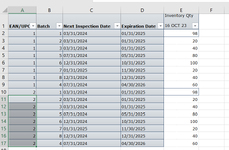
Table 1 "Raw Data" - This is raw data that is pulled giving me EAN/UPC #, the batch, next inspection date, expiration date and unit quantity.
Each EAN/UPC # will have multiple batches and different inspection and expiration dates.
Table 2 "Sls Plan" -Simply just the sales forecast by EAN/UPC by month.
Table 3 "
RawDataPT with Sales
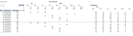
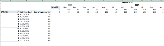
" -A pivot table based on "Raw Data". Bringing in EAN/UPC, expiration date, and unit quantity. Then to the right I did lookup to bring in sales plan for that EAN/UPC #.
Tab 3 "Sls Plan" -Simply just the sales forecast by EAN/UPC by month.
So what I am trying to do is this on the "RawDataPT with Sales" I want to find a way to apply the sales forecast starting in column E row 6 for material 1(50 units). I would want to apply that to the date that expires first. Which is 01/31/205. So in this example for the item that expires on 01/31/2025 I currently have 158 units(cell C8) so for the Nov sales forecast units (50 units) I would want to apply 50 units to 01/31/2025. Then Dec take sales of 60 and apply to balance of the 01/31/2025. Then Jan apply 48 units to 01/31/2025 then use the balance 22 units to the next date that expires next which would be 05/31/2025.
Starting in row 35 i have mocked up a basic idea but not locked into that type of format. It doesn't need to be this format. It can look like anything i just need to apply sales forecast to each material (1 & 2) in this example until it gets to zero to ensure it is sold before it expires. Thank you to anyone that can help
Raw Data
Sales Plan Data
RawDataPT with Sales
Table 1 "Raw Data" - This is raw data that is pulled giving me EAN/UPC #, the batch, next inspection date, expiration date and unit quantity.
Each EAN/UPC # will have multiple batches and different inspection and expiration dates.
Table 2 "Sls Plan" -Simply just the sales forecast by EAN/UPC by month.
Table 3 "
RawDataPT with Sales
" -A pivot table based on "Raw Data". Bringing in EAN/UPC, expiration date, and unit quantity. Then to the right I did lookup to bring in sales plan for that EAN/UPC #.
Tab 3 "Sls Plan" -Simply just the sales forecast by EAN/UPC by month.
So what I am trying to do is this on the "RawDataPT with Sales" I want to find a way to apply the sales forecast starting in column E row 6 for material 1(50 units). I would want to apply that to the date that expires first. Which is 01/31/205. So in this example for the item that expires on 01/31/2025 I currently have 158 units(cell C8) so for the Nov sales forecast units (50 units) I would want to apply 50 units to 01/31/2025. Then Dec take sales of 60 and apply to balance of the 01/31/2025. Then Jan apply 48 units to 01/31/2025 then use the balance 22 units to the next date that expires next which would be 05/31/2025.
Starting in row 35 i have mocked up a basic idea but not locked into that type of format. It doesn't need to be this format. It can look like anything i just need to apply sales forecast to each material (1 & 2) in this example until it gets to zero to ensure it is sold before it expires. Thank you to anyone that can help
Raw Data
| onhandtest.xlsx | |||||||
|---|---|---|---|---|---|---|---|
| A | B | C | D | E | |||
| 1 | EAN/UPC | Batch | Next Inspection Date | Expiration Date | Inventory Qty 16 OCT 23 | ||
| 2 | 1 | 1 | 03/31/2024 | 01/31/2025 | 98 | ||
| 3 | 1 | 2 | 03/31/2024 | 01/31/2025 | 20 | ||
| 4 | 1 | 3 | 03/31/2024 | 01/31/2025 | 40 | ||
| 5 | 1 | 5 | 07/31/2024 | 05/31/2025 | 80 | ||
| 6 | 1 | 6 | 12/31/2024 | 10/31/2025 | 100 | ||
| 7 | 1 | 7 | 01/31/2025 | 11/30/2025 | 20 | ||
| 8 | 1 | 8 | 12/31/2024 | 12/31/2025 | 40 | ||
| 9 | 1 | 4 | 07/31/2024 | 04/30/2026 | 60 | ||
| 10 | 2 | 1 | 03/31/2024 | 01/31/2025 | 98 | ||
| 11 | 2 | 2 | 03/31/2024 | 01/31/2025 | 20 | ||
| 12 | 2 | 3 | 03/31/2024 | 01/31/2025 | 40 | ||
| 13 | 2 | 5 | 07/31/2024 | 05/31/2025 | 80 | ||
| 14 | 2 | 6 | 12/31/2024 | 10/31/2025 | 100 | ||
| 15 | 2 | 7 | 01/31/2025 | 11/30/2025 | 20 | ||
| 16 | 2 | 8 | 12/31/2024 | 12/31/2025 | 40 | ||
| 17 | 2 | 4 | 07/31/2024 | 04/30/2026 | 60 | ||
Invlevel | |||||||
Sales Plan Data
| onhandtest.xlsx | ||||||||||||||||||
|---|---|---|---|---|---|---|---|---|---|---|---|---|---|---|---|---|---|---|
| A | B | C | D | E | F | G | H | I | J | K | L | M | N | O | P | |||
| 1 | Date (Year) | Date (Month) | ||||||||||||||||
| 2 | 2023 | 2024 | ||||||||||||||||
| 3 | Selling Material | Jan | Feb | Mar | Apr | May | Jun | Jul | Aug | Sep | Oct | Nov | Dec | Jan | Feb | Mar | ||
| 4 | 1 | 50 | 60 | 70 | 80 | 90 | 100 | 110 | 120 | 130 | 140 | 150 | 160 | 170 | 180 | 190 | ||
| 5 | 2 | 40 | 60 | 80 | 100 | 120 | 140 | 160 | 180 | 200 | 220 | 240 | 260 | 280 | 300 | 320 | ||
| 6 | ||||||||||||||||||
| 7 | ||||||||||||||||||
Sls Plan | ||||||||||||||||||
RawDataPT with Sales
| onhandtest.xlsx | ||||||||||||||||||||||||||||
|---|---|---|---|---|---|---|---|---|---|---|---|---|---|---|---|---|---|---|---|---|---|---|---|---|---|---|---|---|
| A | B | C | D | E | F | G | H | I | J | K | L | T | U | V | W | X | Y | Z | ||||||||||
| 3 | Sales Forecast | |||||||||||||||||||||||||||
| 4 | 2023 | 2024 | ||||||||||||||||||||||||||
| 5 | EAN/UPC | Nov | Dec | Jan | Feb | Mar | Apr | May | Jun | |||||||||||||||||||
| 6 | 1 | 50 | 60 | 70 | 80 | 90 | 100 | 110 | 120 | |||||||||||||||||||
| 7 | EAN/UPC | Expiration Date | Sum of Inventory Qty | 2 | 40 | 60 | 80 | 100 | 120 | 140 | 160 | 180 | ||||||||||||||||
| 8 | 1 | 01/31/2025 | 158 | |||||||||||||||||||||||||
| 9 | 1 | 04/30/2026 | 60 | |||||||||||||||||||||||||
| 10 | 1 | 05/31/2025 | 80 | |||||||||||||||||||||||||
| 11 | 1 | 10/31/2025 | 100 | |||||||||||||||||||||||||
| 12 | 1 | 11/30/2025 | 20 | |||||||||||||||||||||||||
| 13 | 1 | 12/31/2025 | 40 | |||||||||||||||||||||||||
| 14 | 2 | 01/31/2025 | 158 | |||||||||||||||||||||||||
| 15 | 2 | 04/30/2026 | 60 | |||||||||||||||||||||||||
| 16 | 2 | 05/31/2025 | 80 | |||||||||||||||||||||||||
| 17 | 2 | 10/31/2025 | 100 | |||||||||||||||||||||||||
| 18 | 2 | 11/30/2025 | 20 | |||||||||||||||||||||||||
| 19 | 2 | 12/31/2025 | 40 | |||||||||||||||||||||||||
| 20 | ||||||||||||||||||||||||||||
| 21 | ||||||||||||||||||||||||||||
| 22 | ||||||||||||||||||||||||||||
| 23 | Current idea | Sales Forecast | ||||||||||||||||||||||||||
| 24 | 2023 | 2024 | ||||||||||||||||||||||||||
| 25 | EAN/UPC | Nov | Dec | Jan | Feb | Mar | Apr | May | Jun | Unit Balance | ||||||||||||||||||
| 26 | 1 | 50 | 60 | 70 | 80 | 90 | 100 | 110 | 120 | 2023 | 2024 | |||||||||||||||||
| 27 | 2 | 40 | 60 | 80 | 100 | 120 | 140 | 160 | 180 | Nov | Dec | Jan | Feb | Mar | Apr | |||||||||||||
| 28 | EAN/UPC | Expiration Date | Sum of Inventory Qty | |||||||||||||||||||||||||
| 29 | 1 | 01/31/2025 | 158 | 50 | 60 | 48 | 108 | 48 | 0 | 0 | 0 | 0 | ||||||||||||||||
| 30 | 1 | 04/30/2026 | 60 | 52 | 8 | 60 | 60 | 60 | 60 | 60 | 8 | |||||||||||||||||
| 31 | 1 | 05/31/2025 | 80 | 22 | 58 | 80 | 80 | 58 | 0 | 0 | 0 | |||||||||||||||||
| 32 | 1 | 10/31/2025 | 100 | 22 | 78 | 100 | 100 | 100 | 78 | 0 | 0 | |||||||||||||||||
| 33 | 1 | 11/30/2025 | 20 | 12 | 8 | 20 | 20 | 20 | 20 | 8 | 0 | |||||||||||||||||
| 34 | 1 | 12/31/2025 | 40 | 40 | 40 | 40 | 40 | 40 | 40 | 0 | ||||||||||||||||||
| 35 | 2 | 01/31/2025 | 158 | 40 | 60 | 58 | 118 | 58 | 0 | 0 | 0 | 0 | ||||||||||||||||
| 36 | 2 | 04/30/2026 | 60 | 2 | 58 | 60 | 60 | 60 | 60 | 58 | 0 | |||||||||||||||||
| 37 | 2 | 05/31/2025 | 80 | 22 | 58 | 80 | 80 | 58 | 0 | 0 | 0 | |||||||||||||||||
| 38 | 2 | 10/31/2025 | 100 | 42 | 58 | 100 | 100 | 100 | 58 | 0 | 0 | |||||||||||||||||
| 39 | 2 | 11/30/2025 | 20 | 20 | 20 | 20 | 20 | 20 | 0 | 0 | ||||||||||||||||||
| 40 | 2 | 12/31/2025 | 40 | 40 | 40 | 40 | 40 | 40 | 0 | 0 | ||||||||||||||||||
| 41 | ||||||||||||||||||||||||||||
| 42 | ||||||||||||||||||||||||||||
| 43 | ||||||||||||||||||||||||||||
invlevelPT | ||||||||||||||||||||||||||||
| Cell Formulas | ||
|---|---|---|
| Range | Formula | |
| E6:L6 | E6 | =VLOOKUP($A8,'Sls Plan'!$A:$AE,E1,0) |
| E7:L7 | E7 | =VLOOKUP($D7,'Sls Plan'!$A$4:$Q$5,E1,0) |
| E26:L27 | E26 | =E6 |
| U29:U40 | U29 | =$C29-E29 |
| V29:Z40 | V29 | =U29-F29 |