Look up and match functions

mkvsam

New Member
Joined
Jan 10, 2024
Messages
5
Office Version
  1. 365
  2. 2021
  3. 2019
  4. 2016
  5. 2013
Platform
  1. Windows
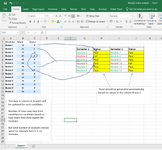
The attached spreadsheet has a list of modules and their corresponding marks and pass or fail status. On the right (two columns that are highlighted in yellow), I need to fill up the status of the modules using look-up and match functions or any other suitable Excel functions.
 

Attachments

  • Module mark analysis.png
    Module mark analysis.png
    158.7 KB · Views: 17

Excel Facts

Copy PDF to Excel
Select data in PDF. Paste to Microsoft Word. Copy from Word and paste to Excel.
Please check:
Book1
GHIJ
3Semester 1StatusSemester 2Status
4Module 1PassModule 7Pass
5Module 2FailModule 8Pass
6Module 3PassModule 9Pass
7Module 4PassModule 10Pass
8Module 5PassModule 11Pass
9Module 6PassModule 12Pass
Sheet1
Cell Formulas
RangeFormula
H4:H9H4=IF(LOOKUP(2,1/($A$2:$A$15=$G4),$C$2:$C$15)="P","Pass","Fail")
J4:J9J4=IF(LOOKUP(2,1/($A$2:$A$15=$I4),$C$2:$C$15)="P","Pass","Fail")

Thanks
 
Upvote 1
Solution
Hello and welcome to MrExcel.

Just comment that in your example module 10 says "Fail", but I think it should say "Pass".

I was building this formula, but @Sam_D_Ben posted before.

varios 10ene2024.xlsm
ABCDEFGHIJ
1ModulesMarkStatus
2Module 170P
3Module 237FSemestre 1StatusSemestre 2Status
4Module 379PModule 1PassModule 7Pass
5Module 445FModule 2FailModule 8Pass
6Module 560PModule 3PassModule 9Pass
7Module 666PModule 4PassModule 10Pass
8Module 266FModule 5PassModule 11Pass
9Module 438PModule 6PassModule 12Pass
10Module 738P
11Module 851P
12Module 953P
13Module 1053P
14Module 1175P
15Module 1261P
16
17
Hoja2
Cell Formulas
RangeFormula
J4:J9,H4:H9H4=IF(INDEX($C$2:$C$15,LOOKUP(2,1/($A$2:$A$15=G4),ROW($A$2:$A$15))-ROW($A$2)+1)="P","Pass","Fail")
 
Upvote 0
Both look up functions work well. How do I solve this problem if I need to pick up electives passed from table 1 to the highlighted cells (gray). As there is no single choice of electives, cell reference for look up is not working. Rather, I need to check the whole list of electives and check which electives the students studied and only pick up passed ones as attached


markss.jpg
 
Upvote 0
Both look up functions work well. How do I solve this problem if I need to pick up electives passed from table 1 to the highlighted cells (gray). As there is no single choice of electives, cell reference for look up is not working. Rather, I need to check the whole list of electives and check which electives the students studied and only pick up passed ones as attached


View attachment 104778
I think this is not possible, as there are three things to do. First, one needs to match third-table items with first-table items. Then check the B or C column cell values. And use the lookup function to capture the status in the second table.
 
Upvote 0
Both look up functions work well. How do I solve this problem if I need to pick up electives passed from table 1 to the highlighted cells (gray).
Try:


varios 10ene2024.xlsm
ABCDEFGHIJ
1ModulesMarkStatus
2Module 170P
3Module 237FSemestre 1StatusSemestre 2Status
4Module 379PModule 1PModule 7P
5Module 445FModule 2FModule 8P
6Module 560PModule 3PModule 9P
7Module 666PModule 4PModule 10P
8Module 266FModule 5PModule 11P
9Efective 120FModule 6PModule 12P
10Module 438PEfectivePEfectiveF
11Module 738P
12Module 851P
13Efective 226F
14Module 953P
15Module 1053P
16Module 1175P
17Module 1261P
18Efective 255P
19Efective 356F
Hoja2
Cell Formulas
RangeFormula
H4:H10H4=INDEX($C$2:$C$19,LARGE(IF(LEFT($A$2:$A$19,LEN(G4))=G4,ROW($A$2:$A$19)),COUNTIF($G$4:$G$10,G4)+COUNTIF($I$4:$I$10,G4))-1)
J4:J10J4=INDEX($C$2:$C$19,LARGE(IF(LEFT($A$2:$A$19,LEN(I4))=I4,ROW($A$2:$A$19)),COUNTIF($I$4:$I$10,I4))-1)
Press CTRL+SHIFT+ENTER to enter array formulas.
 
Upvote 0
Try:


varios 10ene2024.xlsm
ABCDEFGHIJ
1ModulesMarkStatus
2Module 170P
3Module 237FSemestre 1StatusSemestre 2Status
4Module 379PModule 1PModule 7P
5Module 445FModule 2FModule 8P
6Module 560PModule 3PModule 9P
7Module 666PModule 4PModule 10P
8Module 266FModule 5PModule 11P
9Efective 120FModule 6PModule 12P
10Module 438PEfectivePEfectiveF
11Module 738P
12Module 851P
13Efective 226F
14Module 953P
15Module 1053P
16Module 1175P
17Module 1261P
18Efective 255P
19Efective 356F
Hoja2
Cell Formulas
RangeFormula
H4:H10H4=INDEX($C$2:$C$19,LARGE(IF(LEFT($A$2:$A$19,LEN(G4))=G4,ROW($A$2:$A$19)),COUNTIF($G$4:$G$10,G4)+COUNTIF($I$4:$I$10,G4))-1)
J4:J10J4=INDEX($C$2:$C$19,LARGE(IF(LEFT($A$2:$A$19,LEN(I4))=I4,ROW($A$2:$A$19)),COUNTIF($I$4:$I$10,I4))-1)
Press CTRL+SHIFT+ENTER to enter array formulas.
Thanks for your solution. It is not working for me for some reason. I am using 2019 version.
Secondly, I want to update two cells highlighted in gray with electives (from table 1) that the student passed. For example student studied elective 1 and failed. Studied elective 2 and 3 passed. Elective 2 should go to cell G10 and elective 3 should go cell I10 as the student passed these.
 
Upvote 0
Elective 2 should go to cell G10 and elective 3 should go cell I10 as the student passed these.
That is the result presented by the formulas, as you can see in the example I gave, and it also works in 2019, it is the version that I use.

But for it to work you must edit the formula and press the 3 keys at the same time Shift + Control + Enter

;)
 
Upvote 0
That is the result presented by the formulas, as you can see in the example I gave, and it also works in 2019, it is the version that I use.

But for it to work you must edit the formula and press the 3 keys at the same time Shift + Control + Enter

;)
Thanks. But the query is to replace the strings in G10 and I10 cells with the names of the electives (e.g., elective 1, elective 2, etc.) that the student passed from table 1.
 
Upvote 0
Welcome to the MrExcel Message Board!

Cross-posting (posting the same question in more than one forum) is not against our rules, but the method of doing so is covered by #13 of the Forum Rules.

Be sure to follow & read the link at the end of the rule too!

Cross posted at: Match lookup functions
There is no need to repeat the link(s) provided above but if you have posted the question at other places, please provide links to those as well.

If you do cross-post in the future and also provide links, then there shouldn’t be a problem.
 
Upvote 0

Forum statistics

Threads
1,216,027
Messages
6,128,367
Members
449,444
Latest member
abitrandom82

We've detected that you are using an adblocker.

We have a great community of people providing Excel help here, but the hosting costs are enormous. You can help keep this site running by allowing ads on MrExcel.com.
Allow Ads at MrExcel

Which adblocker are you using?

Disable AdBlock

Follow these easy steps to disable AdBlock

1)Click on the icon in the browser’s toolbar.
2)Click on the icon in the browser’s toolbar.
2)Click on the "Pause on this site" option.
Go back

Disable AdBlock Plus

Follow these easy steps to disable AdBlock Plus

1)Click on the icon in the browser’s toolbar.
2)Click on the toggle to disable it for "mrexcel.com".
Go back

Disable uBlock Origin

Follow these easy steps to disable uBlock Origin

1)Click on the icon in the browser’s toolbar.
2)Click on the "Power" button.
3)Click on the "Refresh" button.
Go back

Disable uBlock

Follow these easy steps to disable uBlock

1)Click on the icon in the browser’s toolbar.
2)Click on the "Power" button.
3)Click on the "Refresh" button.
Go back
Back
Top