Looking for some help with this, can not seem to get what I am looking for. I can not get it to calculate the >=
=SUM(SUMIFS(Inventory[Ext-Value],Inventory[Status],{"0"},Inventory[QOH],">="&Inventory[BSL]))
I'm getting the same total as...
=SUMIFS(Inventory[Ext-Value],Inventory[Status],{"0"})
Example of Table: Inventory[Status] = {"0","NS","AP",DP","RB","RBH","MO"}
=SUM(SUMIFS(Inventory[Ext-Value],Inventory[Status],{"0"},Inventory[QOH],">="&Inventory[BSL]))
I'm getting the same total as...
=SUMIFS(Inventory[Ext-Value],Inventory[Status],{"0"})
Example of Table: Inventory[Status] = {"0","NS","AP",DP","RB","RBH","MO"}
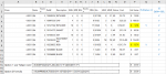
| Store | Make | Source | Part# | Description | QOH | QPR | BSL | Excess | YRSL | Bin | MNS | MNR | Status | Cost | Ext-Value | MfrDet | Return | LastRC | Min | MFRST | Days | TBSL | Entry | New Source | New Bin | Notes |
| 43831 | GM | 3 | 10028352 | RETAINER | 4 | 0 | 0 | 3 | B110G | 8 | 31 | NS | $3.75 | $15.00 | 0Y CPOBK | R | 11/7/2017 | 0 | 5 | 11/4/2017 | 5 |