Lookup Formula

[criner5]

Hi, I'm trying to create a lookup formula that looks at several different criteria.

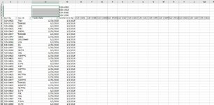
I'm trying to find if there are any formula so that I could in each cell O7-AA7 down the list have True or False appear if for any row the value in column J and column M appear that exist for one of the values in N2:N5 and the acct number listed in O6:AA6.

Any help would be much appreciated.

 

[KRice]

Can you say something more about how the contents of column J factor into the criteria? I see what you mean about finding instances where O6:AA6 match any of the items in N2:N5, but where does column J enter into the criteria...or do you mean column C? Perhaps something like this...

MrExcel20210401.xlsx
	C							J			M	N	O	P	Q	R
1
2												520-14953
3												520-14513
4												520-16182
5												520-12992
6	Acct No							Sec ID			Trade Date	Settlement Date	520-15402	520-16182	520-15408	520-14953
7	520-14953												FALSE	TRUE	FALSE	TRUE
8	123												FALSE	FALSE	FALSE	FALSE
9	520-14513												FALSE	TRUE	FALSE	TRUE
10	789												FALSE	FALSE	FALSE	FALSE
11	520-12992												FALSE	TRUE	FALSE	TRUE
12	1011												FALSE	FALSE	FALSE	FALSE
13	520-16182												FALSE	TRUE	FALSE	TRUE
Sheet4

Cell Formulas
Range	Formula
O7:R13	O7	=AND(ISNUMBER(MATCH(O$6,$N$2:$N$5,0)),ISNUMBER(MATCH($C7,$N$2:$N$5,0)))

 

[criner5]

Can you say something more about how the contents of column J factor into the criteria? I see what you mean about finding instances where O6:AA6 match any of the items in N2:N5, but where does column J enter into the criteria...or do you mean column C? Perhaps something like this...

MrExcel20210401.xlsx
	C							J			M	N	O	P	Q	R
1
2												520-14953
3												520-14513
4												520-16182
5												520-12992
6	Acct No							Sec ID			Trade Date	Settlement Date	520-15402	520-16182	520-15408	520-14953
7	520-14953												FALSE	TRUE	FALSE	TRUE
8	123												FALSE	FALSE	FALSE	FALSE
9	520-14513												FALSE	TRUE	FALSE	TRUE
10	789												FALSE	FALSE	FALSE	FALSE
11	520-12992												FALSE	TRUE	FALSE	TRUE
12	1011												FALSE	FALSE	FALSE	FALSE
13	520-16182												FALSE	TRUE	FALSE	TRUE
Sheet4

Cell Formulas
Range	Formula
O7:R13	O7	=AND(ISNUMBER(MATCH(O$6,$N$2:$N$5,0)),ISNUMBER(MATCH($C7,$N$2:$N$5,0)))

Thank you. I realize my wording was a little confusing.

We want to find out whether rows for account numbers were executed for the same Sec ID on the same day for the account numbers in row O.

So we wanted to create a formula to compare all rows (columns J and M) for the Account Nos. listed in N2:N5 against all rows with account no. in O6 and so on.

For now, we came up with a workaround of separating all the data by account no on separate sheets and then doing a countifs function for each one, but we really need this on one sheet.

 

[Peter_SSs]

What about giving us the sample data again but also include the expected results with detailed explanation of a few of those results?
It would also help greatly if you did that with XL2BB so that helpers don't have to manually type out a huge amount of data to test with.

 

[KRice]

Peter's suggestion is spot on. I'm still not following you, and a working example would be very helpful. I can only guess at the objective. In this example, columns C, J, and M are considered, and we determine where the same set of Acct No, Sec ID, and Trade Date are found on two or more rows AND the Acct No associated with that set is shown in $N$2:$N$5. Then for those rows, the value of TRUE is shown if the column heading in O$6:R$6 has an acct no that matches one listed in $N$2:$N$5...otherwise FALSE is shown.

MrExcel20210401.xlsx
	C							J			M	N	O	P	Q	R
1
2												520-14953
3												520-15402
4												520-16182
5												520-16625
6	Acct No							Sec ID			Trade Date	Settlement Date	520-15402	520-16182	520-16625	520-14953
7	520-16625							TSLX			12/31/2018		FALSE	FALSE	FALSE	FALSE
8	520-10118							9306102			7/1/2018		FALSE	FALSE	FALSE	FALSE
9	520-16625							PSEC			12/31/2018		FALSE	FALSE	TRUE	FALSE
10	520-15402							DIA			10/1/2018		TRUE	FALSE	FALSE	FALSE
11	520-12992							9306102			7/1/2018		FALSE	FALSE	FALSE	FALSE
12	520-15402							DIA			10/1/2018		TRUE	FALSE	FALSE	FALSE
13	520-16625							PSEC			12/31/2018		FALSE	FALSE	TRUE	FALSE
Sheet4

Cell Formulas
Range	Formula
O7:R13	O7	=AND(SUMPRODUCT(($C$7:$C$13=$C7)*($J$7:$J$13=$J7)*($M$7:$M$13=$M7))>=2,ISNUMBER(MATCH($C7,$N$2:$N$5,0)),$C7=O$6)

Cells with Conditional Formatting
Cell	Condition		Cell Format	Stop If True
O7:R13	Cell Value	=TRUE	text	NO