Lookup from multiple columns

[rollingzep]

Hi,

For my sheet, I need to lookup values from two different columns.

Using one column, I get values.

ws.Range("AU2:AU" & ws.Cells(Rows.Count, "Y").End(xlUp).Row).FormulaR1C1 = "=VLOOKUP(""*""&RC[-22]&""*"",HQLA!C1:C35,35,0)"

Also, I need to read it from the Column, C3 of HQLA.

How to use the below along with the above

ws.Range("AU2:AU" & ws.Cells(Rows.Count, "Y").End(xlUp).Row).FormulaR1C1 = "=VLOOKUP(""*""&RC[-22]&""*"",HQLA!C3:C35,35,0)"


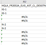
Using C1, I get values like IG-1, N-2.




For missing values, "#N/A",I need it to read from Col, C3.

 

[offthelip]

I think you can just use the iferror function:

ws.Range("AU2:AU" & ws.Cells(Rows.Count, "Y").End(xlUp).Row).FormulaR1C1 = "=iferror(VLOOKUP(""*""&RC[-22]&""*"",HQLA!C1:C35,35,0),VLOOKUP(""*""&RC[-22]&""*"",HQLA!C3:C35,35,0)"

 

[rollingzep]

I think you can just use the iferror function:

ws.Range("AU2:AU" & ws.Cells(Rows.Count, "Y").End(xlUp).Row).FormulaR1C1 = "=iferror(VLOOKUP(""*""&RC[-22]&""*"",HQLA!C1:C35,35,0),VLOOKUP(""*""&RC[-22]&""*"",HQLA!C3:C35,35,0)"

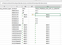
I am still getting the error. I tried using IFNA function too.



'ws.Range("AU2:AU" & ws.Cells(Rows.Count, "Y").End(xlUp).Row).FormulaR1C1 = "=IFERROR(VLOOKUP(""*""&RC[-22]&""*"",HQLA!C1:C35,35,0),VLOOKUP(""*""&RC[-22]&""*"",HQLA!C3:C35,35,0))"

ws.Range("AU2:AU" & ws.Cells(Rows.Count, "Y").End(xlUp).Row).FormulaR1C1 = "=IFNA(VLOOKUP(""*""&RC[-22]&""*"",HQLA!C1:C35,35,0),VLOOKUP(""*""&RC[-22]&""*"",HQLA!C3:C35,35,0))"

 

[rollingzep]

The reason, I am looking from two columns is, if it is 9 digits, it has to lookup to C1 and if it is 12 digits, it does a lookup to Col C3.
If using above IFERROR or IFNA, will the code fill values from C1,where it is 9 digits and and has values like #N/A or #REF!, which is then filled with the lookup to C3, which has 12 digits?

 

[offthelip]

I can see an error in your equation , in the picture you have got:
Vlookup(Y4,HQLA!$C:$AI,35,0)
However column C to AI is only 33 columns, so I think your error is the 35 should be 33.
With the first lookup it starts at column A so 35 is correct.

 

[rollingzep]

I can see an error in your equation , in the picture you have got:
Vlookup(Y4,HQLA!$C:$AI,35,0)
However column C to AI is only 33 columns, so I think your error is the 35 should be 33.
With the first lookup it starts at column A so 35 is correct.

I modified it as you suggested but the result is same

ws.Range("AU2:AU" & ws.Cells(Rows.Count, "Y").End(xlUp).Row).FormulaR1C1 = "=IFNA(VLOOKUP(""*""&RC[-22]&""*"",HQLA!C1:C35,35,0),VLOOKUP(""*""&RC[-22]&""*"",HQLA!C3:C33,33,0))"

 

[offthelip]

What about an alternative approach instead of the iferror or ifna. check the length of column Y:

If(len(Y4) > 9 , vlookup2, vlookup1)

 

[rollingzep]

What about an alternative approach instead of the iferror or ifna. check the length of column Y:

If(len(Y4) > 9 , vlookup2, vlookup1)

How do I loop through the entire col, Y while using the len?

I need to do this using VBA

 

[offthelip]

LEN is an EXCEL function so you can use it in cell of a worksheet. So there is no need to use VBA. I was suggesting using it to combine the two lookup into one cell.
To do the entire column just copy it down.

 

[rollingzep]

LEN is an EXCEL function so you can use it in cell of a worksheet. So there is no need to use VBA. I was suggesting using it to combine the two lookup into one cell.
To do the entire column just copy it down.

I agree but I am using my code for other features in addition to this Vlookup.
That is why I need it in VBA since it has more than 1500 to 2000 rows