Lookup value in table, return the cells above

jgul

New Member
Joined
Aug 26, 2023
Messages
4
Office Version
  1. 365
Platform
  1. Windows
  2. MacOS
Following from .. Lookup value in table, return the cell above
Here is one way (assuming values can only occur once in Column1:Column3)

21 03 23.xlsm
ABCDEF
1Value to SearchResult:Column1Column2Column3
2abcipsumhelloipsumfiller
3defworldworldabctext
4ghiheredefloremhere
5randomwordghi
Cell above
Cell Formulas
RangeFormula
B2:B4B2=INDEX(D:F,AGGREGATE(15,6,ROW(D$2:F$5)/(D$2:F$5=A2),1)-1,AGGREGATE(15,6,(COLUMN(D$2:F$5)-COLUMN(D2)+1)/(D$2:F$5=A2),1))
Hi Peter!
Thanks for that formula. But do you know a way to achive the same workflow, if there is multiple cells with same information.
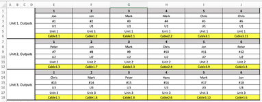
Example the datas in Sheet 1 look like this. The yellow cells will be unique and will not be multiple places. But the other cells will contain simular information.

hjelp.xlsx
ABCDEFGHIJ
1Unit 1, Outputs123456
2JonJonMarkMarkChrisChris
3#1#2#3#4#5#6
4U1U1U1U1U1U1
5Unit 1Unit 1Unit 1Unit 1Unit 1Unit 1
6Cable1.1Cable1.2Cable2.1Cable2.2Cable3.1Cable3.11
7Unit 2, Outputs123456
8PeterJonMarkChrisJonPeter
9#7#8#9#10#11#12
10U2U2U2U2U2U2
11Unit 2Unit 2Unit 2Unit 2Unit 2Unit 2
12Cable1.3Cable1.7Cable2.3Cable2.4Cable3.9Cable3.4
13Unit 3, Outputs123456
14ChrisMarkPeterHansMarkJon
15#13#14#15#16#17#18
16U3U3U3U3U3U3
17Unit 3Unit 3Unit 3Unit 3Unit 3Unit 3
18Cable1.5Cable1.8Cable2.8Cable2.6Cable3.10Cable3.6
Sheet1


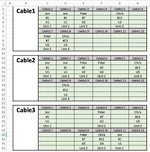
I want to fill out to Sheet 2, that looks like this:

Cell Formulas
RangeFormula
C1,C23,C12C1=RIGHT($B1,20)&"."&"1"
D1,D23,D12D1=RIGHT($B1,20)&"."&"2"
E1,E23,E12E1=RIGHT($B1,20)&"."&"3"
F1,F23,F12F1=RIGHT($B1,20)&"."&"4"
G1,G23,G12G1=RIGHT($B1,20)&"."&"5"
H1,H23,H12H1=RIGHT($B1,20)&"."&"6"
C2:H2,C7:H7,C24:H24,C29:H29,C13:H13,C18:H18C2=IFERROR(INDEX(Sheet1!$E:$J,AGGREGATE(15,6,ROW(Sheet1!$E$1:$J$500)/(Sheet1!$E$1:$J$500=C1),1)-4,AGGREGATE(15,6,(COLUMN(Sheet1!$E$1:$J$500)-COLUMN(Sheet1!$E$1:$J$500)+1)/(Sheet1!$E$1:$J$500=C1),1)),"")
C3:H3,C8:H8,C25:H25,C30:H30,C14:H14,C19:H19C3=IFERROR(INDEX(Sheet1!$E:$J,AGGREGATE(15,6,ROW(Sheet1!$E$1:$J$500)/(Sheet1!$E$1:$J$500=C1),1)-3,AGGREGATE(15,6,(COLUMN(Sheet1!$E$1:$J$500)-COLUMN(Sheet1!$E$1:$J$500)+1)/(Sheet1!$E$1:$J$500=C1),1)),"")
C4:H4,C9:H9,C26:H26,C31:H31,C15:H15,C20:H20C4=IFERROR(INDEX(Sheet1!$E:$J,AGGREGATE(15,6,ROW(Sheet1!$E$1:$J$500)/(Sheet1!$E$1:$J$500=C1),1)-2,AGGREGATE(15,6,(COLUMN(Sheet1!$E$1:$J$500)-COLUMN(Sheet1!$E$1:$J$500)+1)/(Sheet1!$E$1:$J$500=C1),1)),"")
C5:H5,C10:H10,C27:H27,C32:H32,C16:H16,C21:H21C5=IFERROR(INDEX(Sheet1!$E:$J,AGGREGATE(15,6,ROW(Sheet1!$E$1:$J$500)/(Sheet1!$E$1:$J$500=C1),1)-1,AGGREGATE(15,6,(COLUMN(Sheet1!$E$1:$J$500)-COLUMN(Sheet1!$E$1:$J$500)+1)/(Sheet1!$E$1:$J$500=C1),1)),"")
C6,C28,C17C6=RIGHT($B1,20)&"."&"7"
D6,D28,D17D6=RIGHT($B1,20)&"."&"8"
E6,E28,E17E6=RIGHT($B1,20)&"."&"9"
F6,F28,F17F6=RIGHT($B1,20)&"."&"10"
G6,G28,G17G6=RIGHT($B1,20)&"."&"11"
H6,H28,H17H6=RIGHT($B1,20)&"."&"12"


I want all the green cells to be filled out automatically with the search-word in the Grey cell thats right above.

The formula as it is now only fills the first name from sheet 1, in all cells. It looks like it finds the right row but it will return the first column every time.
I need it to be flexible so all cells can be searched for in every formula.
Can someone help? :)
 

Attachments

  • 1693063184653.png
    1693063184653.png
    165.2 KB · Views: 2
  • 1693063261420.png
    1693063261420.png
    231.8 KB · Views: 2
Last edited by a moderator:

Excel Facts

Format cells as time
Select range and press Ctrl+Shift+2 to format cells as time. (Shift 2 is the @ sign).
This was a significantly different question so I have split it to a new thread.
Further, you have a different Excel version to that original OP so have different resources available.

See if this does what you want. The formulas in the green sections only need to go in the top row of each of those sections.
I have also suggested a new formula for the grey sections of Sheet2. These only need to go in column C and the same formula can be copied from C1 to C6, C12, C17 etc

jgul.xlsm
EFGHIJ
1123456
2JonJonMarkMarkChrisChris
3123456
4U1U1U1U1U1U1
5Unit 1Unit 1Unit 1Unit 1Unit 1Unit 1
6Cable1.1Cable1.2Cable2.1Cable2.2Cable3.1Cable3.11
7123456
8PeterJonMarkChrisJonPeter
9789101112
10U2U2U2U2U2U2
11Unit 2Unit 2Unit 2Unit 2Unit 2Unit 2
12Cable1.3Cable1.7Cable2.3Cable2.4Cable3.9Cable3.4
13123456
14ChrisMarkPeterHansMarkJon
15131415161718
16U3U3U3U3U3U3
17Unit 3Unit 3Unit 3Unit 3Unit 3Unit 3
18Cable1.5Cable1.8Cable2.8Cable2.6Cable3.10Cable3.6
19
Sheet1


jgul.xlsm
CDEFGH
1Cable1.1Cable1.2Cable1.3Cable1.4Cable1.5Cable1.6
2JonJonPeter Chris 
312713
4U1U1U2U3
5Unit 1Unit 1Unit 2Unit 3
6Cable1.7Cable1.8Cable1.9Cable1.10Cable1.11Cable1.12
7JonMark    
8814
9U2U3
10Unit 2Unit 3
11
12Cable2.1Cable2.2Cable2.3Cable2.4Cable2.5Cable2.6
13MarkMarkMarkChris Hans
143491016
15U1U1U2U2U3
16Unit 1Unit 1Unit 2Unit 2Unit 3
17Cable2.7Cable2.8Cable2.9Cable2.10Cable2.11Cable2.12
18 Peter    
1915
20U3
21Unit 3
22
23Cable3.1Cable3.2Cable3.3Cable3.4Cable3.5Cable3.6
24Chris  Peter Jon
2551218
26U1U2U3
27Unit 1Unit 2Unit 3
28Cable3.7Cable3.8Cable3.9Cable3.10Cable3.11Cable3.12
29  JonMarkChris 
3011176
31U2U3U1
32Unit 2Unit 3Unit 1
33
Sheet2
Cell Formulas
RangeFormula
C1:H1,C28:H28,C23:H23,C17:H17,C12:H12,C6:H6C1="Cable"&COUNTA(B$1:B1)&"."&SEQUENCE(,6,1+6*(B1=""))
E29:G32,C29:D29,H29,H24:H27,F24:F27,D24:E24,G24,C24:C27,D18:D21,C18,E18:H18,H13:H16,G13,C13:F16,E7:H7,C7:D10,G2:G5,F2,H2,C2:E5C2=LET(c,CHOOSECOLS(Sheet1!$E$2:$J$200,CONCAT(IF(Sheet1!$E$2:$J$200=C1,Sheet1!$E$1:$J$1,""))),IFERROR(INDEX(c,SEQUENCE(4,,MATCH(C1,c,0)-4)),""))
Dynamic array formulas.
 
Last edited:
Upvote 0
Thank you so much for giving your help! We are on a good track to a solution now :)

I have one "small" adjustment, maybe i was a bit diffuse in the question.
The name "Cable" i also want to be flexible. We use different types of cables, the name can be changing and not only "Cable". I really want to write the name for each cable manually in Sheet 2, the B colomn.
So is it possible to in the Sheet 2 use the B1...B12...B23..cell as the key-word, and still be able to copy to get more tables like B45, B56 ans so on..?
And as a bonus question (thats maybe changing with a new formula), here B34 is empty, its filling strange names from C to H and giving "fake" results, is this possible to avoid?

Thank you so much again!
1694253310297.png
 
Upvote 0
Don't really understand. What about the sample data and expected results with XL2BB so it can be copied for testing? Then explain again in relation to that data/results.
 
Upvote 0
Sorry, here.
Sheet 1 is working fine.

So "Sheet 2" contains boxes of 12 outputs. I want to give the names to these boxes manually in "sheet 2".
The name will be in cell B1 + 12 + 23... The name will be changing and if B1= "Name" i want C1 to H1 be like Name.1 , Name.2 up to Name.12. If B1= "DMX" i want C1 to H1 be like DMX.1 , DMX.2 up to DMX.12 have Like i had with my formula, (this can of course be another formula if thats better for a solution). Also if the sequence formula can be adjusted easy to give only 3 or 4 columns it wold be nice. I have added an example for these at the bottom.
I want to be able to copy and add more boxes if needed. One time i use 3, and other times i use maybe 20 boxes. It would also be great if

hjelp.xlsx
ABCDEFGHIJK
1Unit 1, Outputs123456
2JonJonMarkMarkChrisChris
3#1#2#3#4#5#6
4U1U1U1U1U1U1
5Unit 1Unit 1Unit 1Unit 1Unit 1Unit 1
6LK 1.1LK 1.3DMX 1.1DMX 3.1Cable3.1Cable3.11
7Unit 2, Outputs123456
8PeterJonMarkChrisJonPeter
9#7#8#9#10#11#12
10U2U2U2U2U2U2
11Unit 2Unit 2Unit 2Unit 2Unit 2Unit 2
12LK 11.3DMX 11.7LK 12.3Cable2.4LK 13.9DMX 13.4
13Unit 3, Outputs123456
14ChrisMarkPeterHansMarkJon
15#13#14#15#16#17#18
16U3U3U3U3U3U3
17Unit 3Unit 3Unit 3Unit 3Unit 3Unit 3
18Cable1.5DMX 11.8Cable2.8LK 12.6Cable3.10DMX 13.6
19
Sheet1


hjelp.xlsx
ABCDEFGHI
1LK 1Cable1.1Cable1.2Cable1.3Cable1.4Cable1.5Cable1.6
2    Chris 
3#13
4U3
5Unit 3
6Cable1.7Cable1.8Cable1.9Cable1.10Cable1.11Cable1.12
7      
8
9
10
11
12DMX ACable2.1Cable2.2Cable2.3Cable2.4Cable2.5Cable2.6
13   Chris  
14#10
15U2
16Unit 2
17Cable2.7Cable2.8Cable2.9Cable2.10Cable2.11Cable2.12
18 Peter    
19#15
20U3
21Unit 3
22
23Cable 1Cable3.1Cable3.2Cable3.3Cable3.4Cable3.5Cable3.6
24      
25
26
27
28Cable3.7Cable3.8Cable3.9Cable3.10Cable3.11Cable3.12
29   MarkChris 
30#17#6
31U3U1
32Unit 3Unit 1
33
34Cable3.7Cable3.8Cable3.9Cable3.10Cable3.11Cable3.12
35   MarkChris 
36#17#6
37U3U1
38Unit 3Unit 1
39Cable3.7Cable3.8Cable3.9Cable3.10Cable3.11Cable3.12
40   MarkChris 
41#17#6
42U3U1
43Unit 3Unit 1
44
45Cable3.7Cable3.8Cable3.9Cable3.10Cable3.11Cable3.12
46   MarkChris 
47#17#6
48U3U1
49Unit 3Unit 1
50Cable3.7Cable3.8Cable3.9Cable3.10Cable3.11Cable3.12
51   MarkChris 
52#17#6
53U3U1
54Unit 3Unit 1
55
56Cable3.7Cable3.8Cable3.9Cable3.10Cable3.11Cable3.12
57   MarkChris 
58#17#6
59U3U1
60Unit 3Unit 1
61Cable3.7Cable3.8Cable3.9Cable3.10Cable3.11Cable3.12
62   MarkChris 
63#17#6
64U3U1
65Unit 3Unit 1
66
674 BoxCable4.1Cable4.2Cable4.3Cable4.4
68    
69
70
71
72
733 BoxCable5.1Cable5.2Cable5.3
74   
75
76
77
78
Sheet2
Cell Formulas
RangeFormula
C1:H1,C61:H61,C56:H56,C50:H50,C45:H45,C39:H39,C34:H34,C28:H28,C23:H23,C17:H17,C12:H12,C6:H6C1="Cable"&COUNTA(B$1:B1)&"."&SEQUENCE(,6,1+6*(B1=""))
C2,C74,C68,C57,C46,C35,C24,C13C2=LET(c,CHOOSECOLS(Sheet1!$E$2:$J$200,CONCAT(IF(Sheet1!$E$2:$J$200=C1,Sheet1!$E$1:$J$1,""))),IFERROR(INDEX(c,SEQUENCE(4,,MATCH(C1,B1,0)-4)),""))
D2:F2,H2,D74:E74,D68:F68,F62:G65,C62:E62,H62,F57:G60,D57:E57,H57,F51:G54,C51:E51,H51,F46:G49,D46:E46,H46,F40:G43,C40:E40,H40,F35:G38,D35:E35,H35,F29:G32,C29:E29,H29,D24:H24,D18:D21,C18,E18:H18,F13:F16,D13:E13,G13:H13,C7:H7,G2:G5D2=LET(c,CHOOSECOLS(Sheet1!$E$2:$J$200,CONCAT(IF(Sheet1!$E$2:$J$200=D1,Sheet1!$E$1:$J$1,""))),IFERROR(INDEX(c,SEQUENCE(4,,MATCH(D1,c,0)-4)),""))
C67:F67C67="Cable"&COUNTA(B$1:B67)&"."&SEQUENCE(,4,1+6*(B67=""))
C73:E73C73="Cable"&COUNTA(B$1:B73)&"."&SEQUENCE(,3,1+6*(B73=""))
Dynamic array formulas.
 
Upvote 0
Would have been better in Sheet2 to put the expected results as requested, rather than the previous formulas that obviously are not producing the results that you want.

What would you expect in C34 etc where B34 is blank? Or will B34 really have something in it?

Why do the bottom two sections in Sheet2 have less rows and less columns? Will those sections always be that size & therefore require different formulas to the sections above?
Yes so if B34 is empty it would be nice if then C34, D34, E34 also is empty. This is a trifle, because I just can delete these boxes, but it could look strange. If there is results when the box's name is empty. (It will be other people than me using this) If this is hard for the formula to calculate when blank, I can just ignore this and go with it.


The 3 and 4 boxes in the bottom will always have that size and can use one/two different formulas than the 12 boxes. As an template I can have one of each type (12,4,3) and just copy as many as I need.
 
Upvote 0

Forum statistics

Threads
1,215,073
Messages
6,122,974
Members
449,095
Latest member
Mr Hughes

We've detected that you are using an adblocker.

We have a great community of people providing Excel help here, but the hosting costs are enormous. You can help keep this site running by allowing ads on MrExcel.com.
Allow Ads at MrExcel

Which adblocker are you using?

Disable AdBlock

Follow these easy steps to disable AdBlock

1)Click on the icon in the browser’s toolbar.
2)Click on the icon in the browser’s toolbar.
2)Click on the "Pause on this site" option.
Go back

Disable AdBlock Plus

Follow these easy steps to disable AdBlock Plus

1)Click on the icon in the browser’s toolbar.
2)Click on the toggle to disable it for "mrexcel.com".
Go back

Disable uBlock Origin

Follow these easy steps to disable uBlock Origin

1)Click on the icon in the browser’s toolbar.
2)Click on the "Power" button.
3)Click on the "Refresh" button.
Go back

Disable uBlock

Follow these easy steps to disable uBlock

1)Click on the icon in the browser’s toolbar.
2)Click on the "Power" button.
3)Click on the "Refresh" button.
Go back
Back
Top