Lookup with 2 criterias

[feni1388]

Hello...

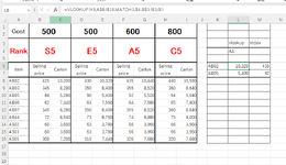
As the image that I uploaded, I need to do a lookup with 2 criterias.
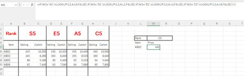
I'm combining if and vlookup together to get the result.
But the thing is that the rank sometimes changes to A4 or A6 and so on.
When the rank changes, I just need to paste a new table but then I also need to change the current formula that I'm using.
Is there any formula that won't need any adjustment even if the rank changes?
If possible, I don't want to use xlookup as there're still some old version of excel in some computers that can't use it.

Thank you.

 

[Cubist]

Would index/match work for you? Your Rank cells are merged so it's hard to say which cell contains the actual text. Adjust B3:I3 as needed.

=INDEX(B6:I0,MATCH(L5,A6:A9,0),MATCH(M3,B3:I3,0))

 

[Peter_SSs]

@Cubist
That isn't a valid formula.

@feni1388
If you want to stick with VLOOKUP see if this works for you.

BTW, I suggest that you investigate XL2BB for providing sample data to make it easier for helpers by not having to manually type out sample data to test with.

24 03 27.xlsm
	A	B	C	D	E	F	G	H	I	J	K	L	M	N
1		S5		E5		A5		C5
2
3													C5
4		Selling	Carton	Selling	Carton	Selling	Carton	Selling	Carton
5												AB02	70
6	AB02	48	61	42	62	89	47	70	91			AB05	91
7	AB03	33	55	54	52	97	31	74	61
8	AB05	77	16	90	93	73	81	91	46
9	AB06	31	95	45	47	74	99	62	82
Price

Cell Formulas
Range	Formula
M5:M6	M5	=VLOOKUP(L5,A$6:I$9,MATCH(M$3,A$1:I$1,0))

 

[Cubist]

@Peter_SSs Can you point out what's wrong?

EDIT I see the range is wrong for I0. Fat fingers. The 0 is next to the 9.

Book2
	A	B	C	D	E	F	G	H	I	J	K	L	M	N
1		B5		E5		A5		C5
2
3													C5
4		Selling	Carton	Selling	Carton	Selling	Carton	Selling	Carton
5												AB02	70
6	AB02	48	61	42	62	89	47	70	91			AB05	91
7	AB03	33	55	54	52	97	31	74	61
8	AB05	77	16	90	93	73	81	91	46
9	AB06	31	95	45	47	74	99	62	82			AB02	70
10												AB05	91
Sheet2

Cell Formulas
Range	Formula
M5:M6	M5	=VLOOKUP(L5,A$6:I$9,MATCH(M$3,A$1:I$1,0))
M9:M10	M9	=INDEX($B$6:$I$9,MATCH(L9,$A$6:$A$9,0),MATCH($M$3,$B$1:$I$1,0))

 

[feni1388]

@Cubist
@Peter_SSs
Thank you both for the solution.
Both solutions works for me.

 

[Peter_SSs]

You're welcome. Glad we could help. Thanks for the follow-up.

 

[feni1388]

@Peter_SSs

As my list is actually longer, I tried a few more items, but the strange thing is that sometimes the result is off.
I don't know why. So I tried Cubist's solution and it's all OK.

 

[Peter_SSs]

@Peter_SSs

As my list is actually longer, I tried a few more items, but the strange thing is that sometimes the result is off.
I don't know why. So I tried Cubist's solution and it's all OK.

As I see it the two formulas should return identical results.
I'd be interested to see some sample data where that happened so I could investigate. Could you provide that, preferably with XL2BB but failing that copy/paste directly into your post?

 

[feni1388]

Cost

500

500

600

800

Rank

S5

E5

A5

C5

A5

vlookup

index

Item

Selling price

Carton

Selling price

Carton

Selling price

Carton

Selling price

Carton

AB02

10,320​

435​

AB05

5,400​

92​

AB02

425​

10,200​

430​

10,320​

435​

10,440​

440​

10,560​

AB03

345​

8,280​

350​

8,400​

355​

8,520​

360​

8,640​

AB05

88​

5,280​

90​

5,400​

92​

5,520​

94​

5,640​

AB06

62​

7,440​

63​

7,560​

64​

7,680​

65​

7,800​

AB07

345​

8,280​

350​

8,400​

355​

8,520​

360​

8,640​

AB44

72​

8,640​

73​

8,760​

74​

8,880​

75​

9,000​

AS02

60​

3,600​

63​

3,780​

66​

3,960​

66​

3,960​

AS03

60​

3,600​

63​

3,780​

66​

3,960​

66​

3,960​

AS05

300​

7,200​

310​

7,440​

320​

7,680​

320​

7,680​

I don't have the original sample anymore so I paste the one that I have now.
Somehow I couldn't make it work with vlookup that you gave me.

 

[Peter_SSs]

Thanks for providing the extra information, sample and image (though using XL2BB would have been better ). The issue is that you have altered one of the ranges incorrectly. The B shown here should be A as it was in my original formula.

With that correction, here are the two formulas again producing the same results. One is not really better than the other, just different ways of approaching the question.

24 03 27.xlsm
	A	B	C	D	E	F	G	H	I	J	K	L	M
1	Cost	500		500		600		800
2
3	Rank	S5		E5		A5		C5
4												A5
5												vlookup	index
6	Item	Selling price	Carton	Selling price	Carton	Selling price	Carton	Selling price	Carton		AB02	435	435
7											AB05	92	92
8	AB02	425	10,200	430	10,320	435	10,440	440	10,560
9	AB03	345	8,280	350	8,400	355	8,520	360	8,640
10	AB05	88	5,280	90	5,400	92	5,520	94	5,640
11	AB06	62	7,440	63	7,560	64	7,680	65	7,800
12	AB07	345	8,280	350	8,400	355	8,520	360	8,640
13	AB44	72	8,640	73	8,760	74	8,880	75	9,000
14	AS02	60	3,600	63	3,780	66	3,960	66	3,960
15	AS03	60	3,600	63	3,780	66	3,960	66	3,960
16	AS05	300	7,200	310	7,440	320	7,680	320	7,680
Price (2)

Cell Formulas
Range	Formula
L6:L7	L6	=VLOOKUP(K6,A$8:I$16,MATCH(L$4,A$3:I$3,0))
M6:M7	M6	=INDEX($B$8:$I$16,MATCH(K6,$A$8:$A$16,0),MATCH($L$4,$B$3:$I$3,0))