Make a formula return a different text when I click on a cell outside of a specified range. (??)

edge37

Board Regular
Joined
Sep 1, 2016
Messages
57
Office Version
  1. 2021
Platform
  1. Windows
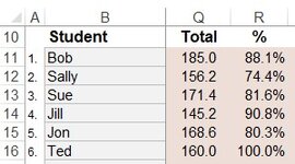
Hello! Given the sample included, I use a VBA code to show the active cell value in a cell (cell AM5), also I need to use the formula:
Code:
=IF(AM5>=91,"Advanced",IF(AM5>=80,"Excellent",IF(AM5>=70,"Needs improvement",IF(AM5<70,"Invalid"))))
so when I click in a name of a student, it returns one of the texts included in the formula based on their grades. The thing is that if I click a blank cell or any other one that is not any of the student's names, it still shows the text "Invalid" because a blank cell is also less than 70.

Is there a way to include something to limit this formula to work only in a range of specified cells (only when i click any student's name) and, if I click another cell outside that range, a specified new text would appear (like "name?" or whatever I choose) in the target cell. Can't figure out this one.

Thanks, and I hope I could describe my problem clearly.
 

Attachments

  • Screenshot_2.jpg
    Screenshot_2.jpg
    19.1 KB · Views: 6
=Try wrapping the VLOOKUPs in an IFERROR (see below). Then both formulas seem to work with your private sub. Of the 2 formulas suggested, I would go with @Scott Huish 's.

Book1
ABMNOPQRSTYZAAAB
1
2
3FORMULAS
4
5   
6
7name?kevin9999's formula
8#STUDENT1010X0.20.451
91ETT0003333$A$1STUDENT?Scott Huish's Formula
102E5YEH0002222
113EG55EG0004444
124G5E0005555
135DFER0000
14
Sheet1
Cell Formulas
RangeFormula
Y5Y5=IFERROR(VLOOKUP($T$8,$B$9:$R$15,15,FALSE),"")
Z5Z5=IFERROR(VLOOKUP($T$8,$B$9:$R$15,16,FALSE),"")
AA5AA5=IFERROR(VLOOKUP($T$8,$B$9:$R$15,17,FALSE),"")
Z7Z7=IF(AA5<>"",IF(AA5>=91,"Advanced",IF(AA5>=80,"Excellent",IF(AA5>=70,"Needs improvement",IF(AA5<70,"Invalid")))),"name?")
T9T9=CELL("address")
Z9Z9=IF(AA5="","STUDENT?",LOOKUP(AA5,{0,70,80,91;"Invalid","Needs Improvement","Excellent","Advanced"}))
P8P8=SUM(C8:N8)/100
P9:P13P9=(C9+D9+E9+F9+G9+H9+I9+J9+K9+L9+M9+N9)
R9:R13R9=SUM(P9:Q9)
 
Upvote 0
Solution

Excel Facts

Add Bullets to Range
Select range. Press Ctrl+1. On Number tab, choose Custom. Type Alt+7 then space then @ sign (using 7 on numeric keypad)
UPDATE I made a tweak on how the value of cell AM5 gets its value and now the formulas work. Thank you so much for your help
 
Upvote 0
=Try wrapping the VLOOKUPs in an IFERROR (see below). Then both formulas seem to work with your private sub. Of the 2 formulas suggested, I would go with @Scott Huish 's.

Book1
ABMNOPQRSTYZAAAB
1
2
3FORMULAS
4
5   
6
7name?kevin9999's formula
8#STUDENT1010X0.20.451
91ETT0003333$A$1STUDENT?Scott Huish's Formula
102E5YEH0002222
113EG55EG0004444
124G5E0005555
135DFER0000
14
Sheet1
Cell Formulas
RangeFormula
Y5Y5=IFERROR(VLOOKUP($T$8,$B$9:$R$15,15,FALSE),"")
Z5Z5=IFERROR(VLOOKUP($T$8,$B$9:$R$15,16,FALSE),"")
AA5AA5=IFERROR(VLOOKUP($T$8,$B$9:$R$15,17,FALSE),"")
Z7Z7=IF(AA5<>"",IF(AA5>=91,"Advanced",IF(AA5>=80,"Excellent",IF(AA5>=70,"Needs improvement",IF(AA5<70,"Invalid")))),"name?")
T9T9=CELL("address")
Z9Z9=IF(AA5="","STUDENT?",LOOKUP(AA5,{0,70,80,91;"Invalid","Needs Improvement","Excellent","Advanced"}))
P8P8=SUM(C8:N8)/100
P9:P13P9=(C9+D9+E9+F9+G9+H9+I9+J9+K9+L9+M9+N9)
R9:R13R9=SUM(P9:Q9)
It works wonderful, thanks again and again
 
Upvote 0

Forum statistics

Threads
1,215,069
Messages
6,122,959
Members
449,096
Latest member
Anshu121

We've detected that you are using an adblocker.

We have a great community of people providing Excel help here, but the hosting costs are enormous. You can help keep this site running by allowing ads on MrExcel.com.
Allow Ads at MrExcel

Which adblocker are you using?

Disable AdBlock

Follow these easy steps to disable AdBlock

1)Click on the icon in the browser’s toolbar.
2)Click on the icon in the browser’s toolbar.
2)Click on the "Pause on this site" option.
Go back

Disable AdBlock Plus

Follow these easy steps to disable AdBlock Plus

1)Click on the icon in the browser’s toolbar.
2)Click on the toggle to disable it for "mrexcel.com".
Go back

Disable uBlock Origin

Follow these easy steps to disable uBlock Origin

1)Click on the icon in the browser’s toolbar.
2)Click on the "Power" button.
3)Click on the "Refresh" button.
Go back

Disable uBlock

Follow these easy steps to disable uBlock

1)Click on the icon in the browser’s toolbar.
2)Click on the "Power" button.
3)Click on the "Refresh" button.
Go back
Back
Top