MODE FORMULA FOR MULTIPLE CONDITIONS??

[michellesssme]

Based on the Data column,
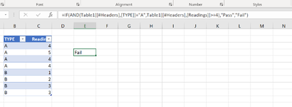
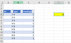
May I know the formula for both conditions (1. & 2.) by using MODE & IF Formula?
1. mode value for condition <650
2. mode value for condition >=650

3. May I know how to insert condition (<650) in the formula (=TEXT(MIN($N:$N),"0")&"~"&TEXT(MAX($N:$N),"0")?
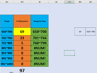
4. How to write the formula to count how many data points fall on the specific range like from 600 to 700?

Data
666
702
741
678
673
707
737
729
797
731
799
729
710
655
608
628
658
643
646
666
628
636
641
677
626
646

 

[michellesssme]

Thanks a lot for the guidance above.
I have another question. May I know what is the formula for automatically detect the highest number in column BH and show in cell BN (69) and the respective range will be along in cell BO (650~700)?

 

[KRice]

Please see my comments in posts #17 and 20 where I mention the inefficiency in taking numeric values and incorporating them into text expressions, and then later extracting those same numeric values from the text expressions for use in subsequent computations. Since you have the source data (originally shown in the range N2:N27) and you seem to be interesting in grouping the data set into bins, is there some reason why using the FREQUENCY function would not work for you? In the example below, the user specifies the thresholds for bins. As one moves down the bin threshold column, each bin threshold and the one immediately above it create a range that the data set is compared to. A count of the number of points falling within each range is produced by the FREQUENCY function (you will need to enter the FREQUENCY formula using Ctrl-Shift-Enter).

I do not understand the purpose or value added by determining the min and max, or the mode and average of the values within each range; however, if that is needed, then the methods described earlier will do that. Another approach that relies directly on the Bin Thresholds is shown below. Also shown is how the FREQUENCY function can be used with other functions to produce the results you asked about (green cells). Also note that I've included the MODE.MULT function in column X. Up until now, the assumption has been that your data will be unimodal (i.e., it has one mode), or if you have multiple modes, only one needs to be returned. If that is not the case, you may want to use MODE.MULT to return all of the modes. In this case, there are four modes (each appears twice in the data set).

I've introduced a named variable "BigNum" to allow some formulas to correctly accept source data in the upper bin where there is no upper bound on the range. The value for BigNum is defined in Formula > Name Manager with =9.99999999999999E+307 in the "Refers to:" field.

MrExcel_20220803.xlsx
	P	Q	R	S	T	U	V	W	X	Y	Z
20	Bin thresholds	Range (a < x <= b)	Data Points in range (frequency)	Min Data Point in Bin Range	Max Data Point in Bin Range	Mode	Average		Multi-Modal	Max frequency	Range
21	600	0~600	0						666	9	600~650
22	650	600~650	9	608	646	628.0	633.6		729
23	700	650~700	7	655	678	666.0	667.6		628
24	750	700~750	8	702	741	729.0	723.3		646
25	800	750~800	2	797	799		798.0
26	850	800~850	0
27		850~	0
Sheet9

Cell Formulas
Range	Formula
R21:R27	R21	=FREQUENCY($N$2:$N$27,$P$21:$P$26)
S21:S27	S21	=IFERROR(AGGREGATE(15,6,($N$2:$N$27)/(($N$2:$N$27>N($P20))*($N$2:$N$27<=MIN($P21,BigNum))),1),"")
T21:T27	T21	=IFERROR(AGGREGATE(14,6,($N$2:$N$27)/(($N$2:$N$27>N($P20))*($N$2:$N$27<=MIN($P21,BigNum))),1),"")
U21:U27	U21	=IFERROR(MODE(IF(($N$2:$N$27>N($P20))*($N$2:$N$27<=MIN($P21,BigNum)),$N$2:$N$27)),"")
V21:V27	V21	=IFERROR(AVERAGE(IF(($N$2:$N$27>N($P20))*($N$2:$N$27<=MIN($P21,BigNum)),$N$2:$N$27)),"")
X21:X24	X21	=MODE.MULT($N$2:$N$27)
Y21	Y21	=MAX(FREQUENCY($N$2:$N$27,$P$21:$P$26))
Z21	Z21	=INDEX($Q$21:$Q$27,MATCH(Y21,$R$21:$R$27,0))
Q21:Q27	Q21	=N(P20)&"~"&P21
Dynamic array formulas.

Source data:

MrExcel_20220803.xlsx
	N
1	Data
2	666
3	702
4	741
5	678
6	673
7	707
8	737
9	729
10	797
11	731
12	799
13	729
14	710
15	655
16	608
17	628
18	658
19	643
20	646
21	666
22	628
23	636
24	641
25	677
26	626
27	646
Sheet9

 

[michellesssme]

Thanks for the comments and guidance, I will consider about it. May I know what is the formula for separate the digit number from the first cell to the 1, 4.7 and 5.2?

1 4.7 5.2	1​	4.7​	5.2​
2 5.4 6.1
3 4.7 5.9

 

[KRice]

There are multiple ways to do that, If for some reason you don't have direct access to the source numbers and are dealing with text strings, and you wanted a formula for this, I would use FILTERXML. In the formula below, I know the delimiter is a single space (because I typed it). It is conceivable that what appears to be a space is not an actual space, in which case you would need to interrogate the text string to determine what the delimiter character is, and then specify that character in the SUBSTITUTE function where " " currently appears:

MrExcel_20220803.xlsx
	A	B	C	D
29	1 4.7 5.2	1	4.7	5.2
30	2 5.4 6.1	2	5.4	6.1
31	3 4.7 5.9	3	4.7	5.9
Sheet9

Cell Formulas
Range	Formula
B29:D31	B29	=TRANSPOSE(FILTERXML( "<t><s>" & SUBSTITUTE( A29, " ", "</s><s>" ) & "</s></t>", "//s" ))
Dynamic array formulas.

If this is to be done only occasionally, you might opt to use the Text to Columns functionality in Excel. Alternatively, you could create a Power Query script to perform this extraction.

8 Ways to Split Text by Delimiter in Excel | How To Excel

www.howtoexcel.org

 

[michellesssme]

There are multiple ways to do that, If for some reason you don't have direct access to the source numbers and are dealing with text strings, and you wanted a formula for this, I would use FILTERXML. In the formula below, I know the delimiter is a single space (because I typed it). It is conceivable that what appears to be a space is not an actual space, in which case you would need to interrogate the text string to determine what the delimiter character is, and then specify that character in the SUBSTITUTE function where " " currently appears:

MrExcel_20220803.xlsx
	A	B	C	D
29	1 4.7 5.2	1	4.7	5.2
30	2 5.4 6.1	2	5.4	6.1
31	3 4.7 5.9	3	4.7	5.9
Sheet9

Cell Formulas
Range	Formula
B29:D31	B29	=TRANSPOSE(FILTERXML( "<t><s>" & SUBSTITUTE( A29, " ", "</s><s>" ) & "</s></t>", "//s" ))
Dynamic array formulas.

If this is to be done only occasionally, you might opt to use the Text to Columns functionality in Excel. Alternatively, you could create a Power Query script to perform this extraction.

8 Ways to Split Text by Delimiter in Excel | How To Excel

www.howtoexcel.org

TQ.
This is my another question about Excel, Kindly informed that my Excel version is 2021.
It shows Fail status after I apply this formula, but suppose the status should be Pass (because all type A readings are more than equal to 4). May I know is there any mistakes from the formula?

 

[KRice]

It isn't clear what you are trying to do. As written, your formula:

=IF(AND(Table1[[#Headers],[TYPE]]="A",Table1[[#Headers],[Reading]]>=4),"Pass","Fail")

...is equivalent to:

=IF(AND("TYPE"="A","Reading">=4),"Pass","Fail")

which will never produce an answer of "Pass" since neither of the conditions is TRUE.. The AND function will always return FALSE. So the first issue is that your structured references include [#Headers], which is why your expression reduces to what I've shown above.
You could change the formula to:

=IF(AND(Table1[TYPE]="A",Table1[Reading]>=4),"Pass","Fail")

which causes the AND function to look at two arrays of TRUEs and FALSEs, but if any single item is FALSE, the formula evaluates to FALSE (see item #3 below). The AND function produces only a single result, not an array.

But what are you trying to evaluate?

1. Do you want 8 answers...one for every pair of type-result?
2. Do you want to know if all 4 "A" types have results >=4...so you want a singe answer for only the A's?
3. Do you want to know if collectively all 8 rows satisfy the condition (so a single instance of a type not being an "A" or a result <4 would be sufficient to produce a single answer of FALSE?

 

[michellesssme]

It isn't clear what you are trying to do. As written, your formula:

=IF(AND(Table1[[#Headers],[TYPE]]="A",Table1[[#Headers],[Reading]]>=4),"Pass","Fail")

...is equivalent to:

=IF(AND("TYPE"="A","Reading">=4),"Pass","Fail")

which will never produce an answer of "Pass" since neither of the conditions is TRUE.. The AND function will always return FALSE. So the first issue is that your structured references include [#Headers], which is why your expression reduces to what I've shown above.
You could change the formula to:

=IF(AND(Table1[TYPE]="A",Table1[Reading]>=4),"Pass","Fail")

which causes the AND function to look at two arrays of TRUEs and FALSEs, but if any single item is FALSE, the formula evaluates to FALSE (see item #3 below). The AND function produces only a single result, not an array.

But what are you trying to evaluate?

1. Do you want 8 answers...one for every pair of type-result?
2. Do you want to know if all 4 "A" types have results >=4...so you want a singe answer for only the A's?
3. Do you want to know if collectively all 8 rows satisfy the condition (so a single instance of a type not being an "A" or a result <4 would be sufficient to produce a single answer of FALSE?

I want a status (PASS/FAIL) for each TYPE
if [TYPE]="A" and [Readings]>= 4 then "pass" else "fail"
if [TYPE]="B" and [Readings]>= 4 then "pass" else "fail"
Am I stated clearly?

 

[KRice]

No, that's not entirely clear. Why do you want to put the "Type" in the expression? Are there only two types, A or B?...or is there some possibility that three or more types are present?
Based on what you've described, why wouldn't this work:

=IF(Table1[@Readings]>=4,"Pass","Fail")

 

[michellesssme]

No, that's not entirely clear. Why do you want to put the "Type" in the expression? Are there only two types, A or B?...or is there some possibility that three or more types are present?
Based on what you've described, why wouldn't this work:

=IF(Table1[@Readings]>=4,"Pass","Fail")

thanks again for the provided formula.
I have another question.
May I know what is the formula to make the yellow cell show 9 (Column No.) and it is clickable (I want to make it clickable as the table is in different sheet)?
*it shows 9 as the reading for No.9 is less than 2.

 

[KRice]

I'm not sure what you want to do. Do you want a formula to return the value in the [No] column if the value in the [readings] column is less than 2? What do you want to see if multiple values in the [readings] column are less than 2? A formula will return the results automatically, so no further user interaction would be necessary. What does "clickable" mean?