Modify VBA code to sort by date ignoring words, please :)

[dakotacondon1]

Hi! I have data that looks like this:

Axon Body 3 Video 2021-11-25 2229 X60A986468J

Axon Body 3 Video 2021-11-24 2231 X60A656565V

Axon Fleet 3 Interior Camera Video 2022-02-21 1920 X60A656565V

Axon Body 3 Video 2021-08-26 2158 X60A656565V

Axon Fleet 3 Front Camera Video 2021-11-27 2156 X60A986468J

Axon Body 3 Video 2021-12-01 2154 X60A656565V

(These are not real, I made them up.)

Ultimately, I need these titles to be ordered chronologically and bracketed with a space in the middle in one cell so they can be pasted into a report. The end result should look like this:

[Axon Body 3 Video 2021-08-26 2158 X60A656565V] [Axon Body 3 Video 2021-11-24 2231 X60A656565V] [Axon Body 3 Video 2021-11-25 2229 X60A986468J] [Axon Fleet 3 Front Camera Video 2021-11-27 2156 X60A986468J] [Axon Body 3 Video 2021-12-01 2154 X60A656565V] [Axon Fleet 3 Interior Camera Video 2022-02-21 1920 X60A656565V]

I do not understand VBA code. I hope to one day but right now I am just an okay Google-er. Currently, I have it miraculously set up with VBA code I found on the internet so when you paste the data into Column B, it automatically orders it. The problem is that it is ordering it alphabetically so it obviously doesn't work when there are any differences in the beginnings of the titles. I need these to be ordered by the date and then the time (military time, the four numbers after the date) no matter the title. And then they will work with the rudimentary formulas I made to make them formatted correctly.

Right now I have this in a Worksheet - Change situation:

Sub Worksheet_Change(ByVal Target As Range)

Dim lastrow As Long
lastrow = Cells(Rows.Count, 2).End(xlUp).Row

    If Not Intersect(Target, Range("B:B")) Is Nothing Then
        Range("B1:B" & lastrow).Sort key1:=Range("B1:B" & lastrow), _
        order1:=xlAscending, Header:=xlYes

    
    End If
    End Sub

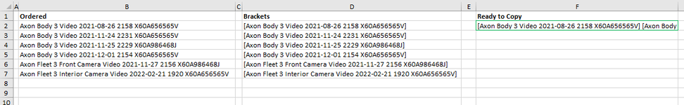
Then Column B adds brackets [=IF(B2<>"", "["&B2&"]", " "] and then Column F puts them all together in one cell and adds spaces [=D2&" "&D3&" "&D4&" "&D5&" "&D6&" "&D7&" "&D8.....etc]

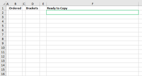
I'm not sure if I am totally making sense to people who actually know how this works. I have attached a screenshot of the sheet before pasting and one after pasting the above values in it.

Please be nice I have no idea what I am doing and THANK YOU

 

[rlv01]

One example.

Book2
	A	B	C
1	Data	Helper Column (date)	Result
2	Axon Body 3 Video 2021-08-26 2158 X60A656565V	2021-08-26 21:58	[Axon Body 3 Video 2021-08-26 2158 X60A656565V] [Axon Body 3 Video 2021-11-24 2231 X60A656565V] [Axon Body 3 Video 2021-11-25 2229 X60A986468J] [Axon Fleet 3 Front Camera Video 2021-11-27 2156 X60A986468J] [Axon Body 3 Video 2021-12-01 2154 X60A656565V] [Axon Fleet 3 Interior Camera Video 2022-02-21 1920 X60A656565V]
3	Axon Body 3 Video 2021-11-24 2231 X60A656565V	2021-11-24 22:31
4	Axon Body 3 Video 2021-11-25 2229 X60A986468J	2021-11-25 22:29
5	Axon Fleet 3 Front Camera Video 2021-11-27 2156 X60A986468J	2021-11-27 21:56
6	Axon Body 3 Video 2021-12-01 2154 X60A656565V	2021-12-01 21:54
7	Axon Fleet 3 Interior Camera Video 2022-02-21 1920 X60A656565V	2022-02-21 19:20
Sheet1

Cell Formulas
Range	Formula
B2:B7	B2	=DATEVALUE(MID(A2,FIND("202",A2),10))+TIME(LEFT(MID(A2,FIND("202",A2)+11,4),2),RIGHT(MID(A2,FIND("202",A2)+11,4),2),0)

Sub Worksheet_Change(ByVal Target As Range)
    Dim rng As Range
    Dim R As Range
    Dim S As String

    If Not Intersect(Target, Range("A:A")) Is Nothing Then
        With Me
            Set rng = .Range("A2:B" & .Range("A" & .Rows.Count).End(xlUp).Row)
            rng.Sort key1:=.Range("B2"), order1:=xlAscending, Header:=xlNo

            For Each R In rng.Resize(, 1)
                S = S & "[" & R.Value & "] "
            Next R

            With .Range("C2")
                .Value = Trim(S)
                .WrapText = True
            End With
        End With
    End If
End Sub

 

[Herakles]

I am now realizing that you maybe meant this as a partner to the VBA code and that have to work together? Not sure how to alter that to fit this magic in...

All the VBA code does that you posted is sort the data in column B when cell in column changes value.

My formulas split out the data and MT to enable a chronilogical sort to be carried out.

I would question whether you actually want to do this each and every time.

Why not just do it when you need to report on the data.

What will users get out of looking at the concatenated data in one cell?

My post puts the data in Column A so just change the column reference in the formulas to B.

 

[dakotacondon1]

One example.

Book2
	A	B	C
1	Data	Helper Column (date)	Result
2	Axon Body 3 Video 2021-08-26 2158 X60A656565V	2021-08-26 21:58	[Axon Body 3 Video 2021-08-26 2158 X60A656565V] [Axon Body 3 Video 2021-11-24 2231 X60A656565V] [Axon Body 3 Video 2021-11-25 2229 X60A986468J] [Axon Fleet 3 Front Camera Video 2021-11-27 2156 X60A986468J] [Axon Body 3 Video 2021-12-01 2154 X60A656565V] [Axon Fleet 3 Interior Camera Video 2022-02-21 1920 X60A656565V]
3	Axon Body 3 Video 2021-11-24 2231 X60A656565V	2021-11-24 22:31
4	Axon Body 3 Video 2021-11-25 2229 X60A986468J	2021-11-25 22:29
5	Axon Fleet 3 Front Camera Video 2021-11-27 2156 X60A986468J	2021-11-27 21:56
6	Axon Body 3 Video 2021-12-01 2154 X60A656565V	2021-12-01 21:54
7	Axon Fleet 3 Interior Camera Video 2022-02-21 1920 X60A656565V	2022-02-21 19:20
Sheet1

Cell Formulas
Range	Formula
B2:B7	B2	=DATEVALUE(MID(A2,FIND("202",A2),10))+TIME(LEFT(MID(A2,FIND("202",A2)+11,4),2),RIGHT(MID(A2,FIND("202",A2)+11,4),2),0)

Sub Worksheet_Change(ByVal Target As Range)
    Dim rng As Range
    Dim R As Range
    Dim S As String

    If Not Intersect(Target, Range("A:A")) Is Nothing Then
        With Me
            Set rng = .Range("A2:B" & .Range("A" & .Rows.Count).End(xlUp).Row)
            rng.Sort key1:=.Range("B2"), order1:=xlAscending, Header:=xlNo

            For Each R In rng.Resize(, 1)
                S = S & "[" & R.Value & "] "
            Next R

            With .Range("C2")
                .Value = Trim(S)
                .WrapText = True
            End With
        End With
    End If
End Sub

I mean c'mon, this is magic. This is EXACTLY right! Thank you x1,000. Very dumb follow-up question because I don't want to break it - what would be the best way to clear this? I tried Clear Contents on everything below the header in column A, and it puts "[Data] []" in the result box, if I Clear Contents on the whole column, it has two empty brackets in the result box: "[] []". I would like to have a header on that column but make it easy for other people to reset it - thoughts?

 

[rlv01]

Ok, what about something like this.

Sub Worksheet_Change(ByVal Target As Range)
    Dim rng As Range
    Dim R As Range
    Dim S As String

    If Not Intersect(Target, Range("A:A")) Is Nothing Then
        With Me
            Set rng = .Range("A2:B" & .Range("A" & .Rows.Count).End(xlUp).Row)
            rng.Sort key1:=.Range("B2"), order1:=xlAscending, Header:=xlNo

            For Each R In rng.Resize(, 1)
                S = S & "[" & R.Value & "] "
            Next R

            With .Range("C2")
                If Left(S, 5) = "[Data" Then
                    S = ""
                End If
                .Value = Trim(S)
                .WrapText = True
            End With
        End With
    End If
End Sub

 

[dakotacondon1]

Ok, what about something like this.

Sub Worksheet_Change(ByVal Target As Range)
    Dim rng As Range
    Dim R As Range
    Dim S As String

    If Not Intersect(Target, Range("A:A")) Is Nothing Then
        With Me
            Set rng = .Range("A2:B" & .Range("A" & .Rows.Count).End(xlUp).Row)
            rng.Sort key1:=.Range("B2"), order1:=xlAscending, Header:=xlNo

            For Each R In rng.Resize(, 1)
                S = S & "[" & R.Value & "] "
            Next R

            With .Range("C2")
                If Left(S, 5) = "[Data" Then
                    S = ""
                End If
                .Value = Trim(S)
                .WrapText = True
            End With
        End With
    End If
End Sub

Amazing - yes! This functions PERFECTLY. Thank you, again!!!!!!