thetnaingsoe
New Member
- Joined
- Nov 7, 2018
- Messages
- 7
- Office Version
- 365
- Platform
- Windows
Hey everyone,
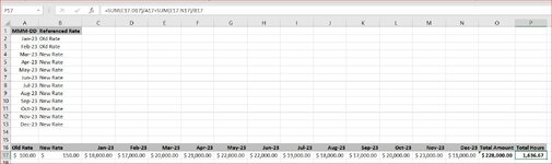
I have a table which defines what rate to be applied to each period (from cell A1 to B13).
In Row 16 and 17, there is old rate (cell A17) and new rate (cell B17). From cell C17 to N18 is monthly revenue.
Rate table defines that Jan 2023 and Feb 2023 are using the old rate and Mar 2023 to Dec 2023 are using the new rate.
Cell P17 will calculate the total hours for the year. Since Jan and Feb 2023 are using the old rates, revenue from that 2 periods are converted to hours using the old rate and Mar to Dec 2023 revenues are converted to hours using the new rate. Manual calculation will look like this =SUM(C17:D17)/A17+SUM(E17:N17)/B17
Is there a way to automate this calculation?
Thanks in advance!