I need a formula to find the most ideal row and displays that row's column 1 value.
To evaluate a row, I place the highest priority on it having the lowest value in column 3. (MIN(M3:M10)
If there is only 1 row with this lowest value then I display the value from column 1. INDEX(K3:K10,MATCH(MIN(M3:M10),M3:M10,0))
If there is more than 1 row with the lowest value in column 3 then the formula takes those rows and prioritizes the lowest value in column 2.
Again, if there is more than 1 row that meets the criteria (lowest value in column 2) I then need it to prioritize the value closest to 1 in column 1.
In the end, the formula should display the value of column 1 in the most suitable row.
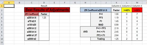
In my example image, the formula would look at column 3: find row 5, row 7, and row 10 each having the lowest value (4).
It would then look at column 2: find row 7 and 10 each having the lowest value (2).
It would then look at column 1: find that row 10 has the closest value to 1 (1.25).
Finally it would display the value of column 1 of the ideal row.
The desired result in my example image is 1.25.
I'm struggling to find the correct way to structure the formula or even how to have it evaluate subsets of data.
To evaluate a row, I place the highest priority on it having the lowest value in column 3. (MIN(M3:M10)
If there is only 1 row with this lowest value then I display the value from column 1. INDEX(K3:K10,MATCH(MIN(M3:M10),M3:M10,0))
If there is more than 1 row with the lowest value in column 3 then the formula takes those rows and prioritizes the lowest value in column 2.
Again, if there is more than 1 row that meets the criteria (lowest value in column 2) I then need it to prioritize the value closest to 1 in column 1.
In the end, the formula should display the value of column 1 in the most suitable row.
In my example image, the formula would look at column 3: find row 5, row 7, and row 10 each having the lowest value (4).
It would then look at column 2: find row 7 and 10 each having the lowest value (2).
It would then look at column 1: find that row 10 has the closest value to 1 (1.25).
Finally it would display the value of column 1 of the ideal row.
The desired result in my example image is 1.25.
I'm struggling to find the correct way to structure the formula or even how to have it evaluate subsets of data.