Multiple Vlookup's with ISNA (multiple columns)

[Seintje]

Good evening,
I am struggling with a formula and the result I get is #N/A.
The point I need to look in one tab in multiple columns.

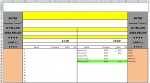
So I need to look up information in column C3 until E40 and L3 until N44 and U3 until W44 and AD3 until AF44
the value in the 3rd column is what it needs to show.

The single formula as below works fine, which is:
=IF(ISNA(VLOOKUP(N17,MATRIX!$C$2:$E$114,3,0))," ",(VLOOKUP(N17,MATRIX!$C$2:$E$114,3,0)))

Then I tried to following step:
=IF(ISNA(VLOOKUP(N17,MATRIX!$C$3:$E$22,3,0)),IF(ISNA(VLOOKUP(N17,MATRIX!$L$3:$N$44,3,0)),"",(VLOOKUP(N17,MATRIX!$C$3:$E$22,3,0))),(VLOOKUP(N17,MATRIX!$L$3:$N$44,3,0)))

This results in #N/A

Can anyone help me a bit futher.
Thank you


.

 

[Dave87]

=IFERROR(VLOOKUP(N17,Matrix!$C$3:$E$22,3,FALSE),IFERROR(VLOOKUP(N17,Matrix!$L$3:$N$44,3,0),IFERROR(VLOOKUP(N17,Matrix!$U$3:$W$44,3,0),VLOOKUP(N17,Matrix!$AD$3:$AF$44,3,0))))

Try this, if it doesnt work can you post data in XL2BB or screenshots/table

 

[Seintje]

Good morning,

Thanks for the quick reply, unfortunately it didn't work.
To explain a bit more

Capture 1
In the orange field I type a name* in column N.
The formula in column L needs to search in the Tab Matrix (Capture 2) on all levels

for example:
In capture 1 I highlighted "working result" in Green.
The formula in column L is working
=IF(ISNA(VLOOKUP(N19,MATRIX!C3:E22,3,0))," ",(VLOOKUP(N19,MATRIX!C3:E22,3,0)))
This formula is looking at Tab "Matrix", column C3,until E22 (see Capture 2)
the result is 222A

The goal is now to create a formula which looks in column C3 until E22 & C25 until E44 & L3 until N44 & U3 until W44 & AD3 until AF44 (see capture 2)
So, that works, "Kees de Test" in (capture 1) should give a result 304A.

Hope this makes it more clear.

 

[Dave87]

this works for me when i test it (paste in L15 and copy down)

=IFERROR(VLOOKUP(N15,Matrix!$C$3:$E$22,3,FALSE),IFERROR(VLOOKUP(N15,Matrix!$L$3:$N$44,3,FALSE),IFERROR(VLOOKUP(N15,Matrix!$U$3:$W$44,3,FALSE),VLOOKUP(N15,Matrix!$AD$3:$AF$44,3,FALSE))))

 

[Seintje]

You're the greatest!!!
It's works.
Fantastic, thank you very much for you quick help.

Regards,
Erik

 

[Seintje]

Sorry, one more small question.
When the N is empty is give a #N/A instead of leaving it empty. (see capture 3)

any solution for that?

 

[Seintje]

I have done some more research but still can't find the solution.
I have tried the following formula to get rid of the #N/A but it gives me following error. (You've entered too many arguments in this function)
Instead of N/A the cell should be stay blank.

=IFERROR(VLOOKUP(N18,MATRIX!$C$3:$E$22,3,FALSE),IFERROR(VLOOKUP(N18,MATRIX!$L$3:$N$44,3,FALSE),IFERROR(VLOOKUP(N18,MATRIX!$U$3:$W$44,3,FALSE),VLOOKUP(N18,MATRIX!$AD$3:$AF$44,3,FALSE), " ")))

Does anyone have an idea what I do wrong?
Your help is much appreciated.

 

[Dave87]

in L15 paste
=IFERROR(IFERROR(VLOOKUP(N15,Matrix!$C$3:$E$22,3,FALSE),IFERROR(VLOOKUP(N15,Matrix!$L$3:$N$44,3,FALSE),IFERROR(VLOOKUP(N15,Matrix!$U$3:$W$44,3,FALSE),VLOOKUP(N15,Matrix!$AD$3:$AF$44,3,FALSE)))),"")

the " " at the end of your formula doesnt have a corresponding iferror at the start, its just stuck on there so Excel doesnt know what to do with it

 

[Seintje]

Thanks, I have tested it and it works.
Thanks a lot.