Narrowing a list based on latest year & valid score field

PNuff

New Member
Joined
Dec 6, 2017
Messages
7
Office Version
  1. 365
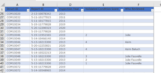
Hi - I have a list of a about 150K line items, each with 5 cols as shown below. The Struct_ID (Col. A) represents a pipe and the rest of the cols are records of past inspections that have been done on that particular pipe. I'm looking to narrow down the list to include only the entries with the lastest inspection data and that include a Validated Condition Score. This would mean that, in my final list, there is only one entry for each Struct_ID. You'll note that currently, one Struct_ID could have multiple entries. Ex COM10046 (ln 32, 33 & 34) has three entries. These three lines represent inspections that were done in years 2019, 2014 and 2013. I'm hoping to extract the line with the lastest year, and that has an actual number in Col E "Validated Condition Score". In the case of COM10046, the "chosen" line would be L32 bc it is the latest year (2019) with an actual "Validated Condition Score".
There are probably several thousand occurences of Struct_ID's with multiple entries, but for all of them, there are no more than 10 entries for each 'multiple'. Many Struct_ID's do not have multiple entries. Single entry Struct_IDs (with a Validated Construction Score) are desired to be included in the final list. For multiple entries or single entries, I am only interested in those entries with a Validated Condition Score. Entries, single or multiple, with no Validated Condition Score do not need to be included. I envision the list to go from 150k entries to under 100k entries...
If it helps, it would be easy to construct another column and have a field generated 'toggle' ( "chosen" / "not chosen") for the chosen line item, and I can sort & extract the final list from that. It does not need to be dynamic...it is a one time operation. The final list should include all 5 original column data. The intent is for the final list to be used as a Vlookup table in another spreadsheet.
In the case of a multiple line entry of Struct ID that has the same Inspection Year, then the larger "Validated Condition Score" would get "chosen'.
Validated Condition Score include: 0,1,2,3,4,5. The Col includes "blanks", but these are nota valid score.

I believe I have covered everything, but I'll be online to provide additional clarity if required. Any help you could provide would be appreciated!

Thanks again!

Pete

1661440005011.png
 

Attachments

  • 1661439937925.png
    1661439937925.png
    90 KB · Views: 6

Excel Facts

How can you automate Excel?
Press Alt+F11 from Windows Excel to open the Visual Basic for Applications (VBA) editor.
How about this, using Power Query.

Book3
ABCDEFGHIJK
1Struct IDReport IDInspection YearValidated Condition ScoreWho ReviewedStruct IDReport IDInspection YearValidated Condition ScoreWho Reviewed
2COM100202-13-100783422013COM100202-13-100783422013
3COM100325-11-101778152011COM100325-11-101778152011
4COM100335-11-101778152011COM100335-11-101778152011
5COM100345-19-117798282019COM100345-19-117798282019
6COM100355-20-122003232020COM100355-20-122003232020
7COM100355-19-117798282019COM100465-19-1195156520192Julie
8COM100465-19-1195156520192JulieCOM100475-20-122538212020
9COM100465-14-104661402014COM100485-14-105222132014
10COM100465-13-1021530020134AsimCOM100495-13-1021530020132Julie
11COM100475-20-122538212020COM100705-13-1021530020131Julie
12COM100475-13-1021530020134AsimCOM100725-19-117798282019
13COM100485-14-105222132014
14COM100485-13-1021530020133Julie
15COM100495-13-1021530020132Julie
16COM100705-13-1021530020131Julie
17COM100725-19-117798282019
18COM100725-14-105489652014
Sheet1


Power Query:
let
    Source = Excel.CurrentWorkbook(){[Name="Table1"]}[Content],
    Group = Table.Group(Source, {"Struct ID"}, {{"Data", each _, type table [Struct ID=text, Report ID=text, Inspection Year=number, Validated Condition Score=nullable number, Who Reviewed=nullable text]}}),
    Last = Table.TransformColumns(Group,{{"Data", each Table.LastN(Table.Sort(_, {"Inspection Year"}),1)}}),
    Expand = Table.ExpandTableColumn(Last, "Data", {"Report ID", "Inspection Year", "Validated Condition Score", "Who Reviewed"}, {"Report ID", "Inspection Year", "Validated Condition Score", "Who Reviewed"})
in
    Expand
 
Upvote 0
It would be helpful if you updated your account details to include what version of Excel you are using. For example, if you're on 365, you could do this.

Book3
ABCDEFGHIJKL
1Struct IDReport IDInspection YearValidated Condition ScoreWho ReviewedStruct IDReport IDInspection YearValidated Condition ScoreWho Reviewed
2COM100202-13-100783422013COM100202-13-100783422013
3COM100325-11-101778152011COM100325-11-101778152011
4COM100335-11-101778152011COM100335-11-101778152011
5COM100345-19-117798282019COM100345-19-117798282019
6COM100355-20-122003232020COM100355-20-122003232020
7COM100355-19-117798282019COM100465-19-1195156520192Julie
8COM100465-19-1195156520192JulieCOM100475-20-122538212020
9COM100465-14-104661402014COM100485-14-105222132014
10COM100465-13-1021530020134AsimCOM100495-13-1021530020132Julie
11COM100475-20-122538212020COM100705-13-1021530020131Julie
12COM100475-13-1021530020134AsimCOM100725-19-117798282019
13COM100485-14-105222132014
14COM100485-13-1021530020133Julie
15COM100495-13-1021530020132Julie
16COM100705-13-1021530020131Julie
17COM100725-19-117798282019
18COM100725-14-105489652014
Sheet1
Cell Formulas
RangeFormula
H2:L12H2=LET(sID,Table3[Struct ID],y,Table3[Inspection Year],u,UNIQUE(sID),m,MAXIFS(y,sID,u),x,ISNUMBER(MATCH(sID&y,u&m,0)),FILTER(Table3,x))
Dynamic array formulas.
Thanks - I've updated my account...it is indeed Microsoft 365 Apps :). I'm not familiar with Power Query...is it an add-on?
 
Upvote 0
Another option
Fluff.xlsm
ABCDEFGHIJKL
1Struct IDReport IDInspection YearValidated Condition ScoreWho ReviewedStruct IDReport IDInspection YearValidated Condition ScoreWho Reviewed
2COM100202-13-100783422013COM100465-13-1021530020194Asim
3COM100325-11-101778152011COM100475-13-1021530020134Asim
4COM100335-11-101778152011COM100485-14-1052221320141b
5COM100345-19-117798282019COM100495-13-1021530020132Julie
6COM100355-20-122003232020COM100705-13-1021530020131Julie
7COM100355-19-117798282019
8COM100465-19-1195156520192Julie
9COM100465-14-104661402014
10COM100465-13-1021530020194Asim
11COM100475-20-122538212020
12COM100475-13-1021530020134Asim
13COM100485-14-1052221320141b
14COM100485-13-1021530020133Julie
15COM100495-13-1021530020132Julie
16COM100705-13-1021530020131Julie
17COM100725-19-117798282019
18COM100725-14-105489652014
Data
Cell Formulas
RangeFormula
H2:L6H2=LET(f,FILTER(A2:E500,D2:D500<>""),s,SEQUENCE(ROWS(f)),u,UNIQUE(INDEX(f,,1)),b,BYROW(u,LAMBDA(br,CONCAT(INDEX(SORT(FILTER(INDEX(f,s,{3,4}),INDEX(f,,1)=br),{1,2},-1),1,{1,2})))),FILTER(f,ISNUMBER(MATCH(INDEX(f,,1)&INDEX(f&"",,3)&INDEX(f&"",,4),u&b,0))))
Dynamic array formulas.
 
Upvote 0
Another option if there are not too many filtered rows
Excel Formula:
=LET(f,SORT(FILTER(A2:E500,D2:D500<>""),{1,3,4},{1,-1,-1}),r,ROWS(f),FILTER(f,MMULT((SEQUENCE(r)>=SEQUENCE(,r))*(INDEX(f,,1)=TRANSPOSE(INDEX(f,,1))),SEQUENCE(r,,,0))=1))

And if you do have a lot of filtered rows
Excel Formula:
=LET(f,SORT(FILTER(A2:E25000,D2:D25000<>""),{1,3,4},{1,-1,-1}),s,SEQUENCE(ROWS(f)),b,BYROW(UNIQUE(INDEX(f,,1)),LAMBDA(br,MIN(IF(br=INDEX(f,,1),s)))),FILTER(f,ISNUMBER(MATCH(s,b,0))))
 
Last edited:
Upvote 0

Forum statistics

Threads
1,215,437
Messages
6,124,871
Members
449,192
Latest member
MoonDancer

We've detected that you are using an adblocker.

We have a great community of people providing Excel help here, but the hosting costs are enormous. You can help keep this site running by allowing ads on MrExcel.com.
Allow Ads at MrExcel

Which adblocker are you using?

Disable AdBlock

Follow these easy steps to disable AdBlock

1)Click on the icon in the browser’s toolbar.
2)Click on the icon in the browser’s toolbar.
2)Click on the "Pause on this site" option.
Go back

Disable AdBlock Plus

Follow these easy steps to disable AdBlock Plus

1)Click on the icon in the browser’s toolbar.
2)Click on the toggle to disable it for "mrexcel.com".
Go back

Disable uBlock Origin

Follow these easy steps to disable uBlock Origin

1)Click on the icon in the browser’s toolbar.
2)Click on the "Power" button.
3)Click on the "Refresh" button.
Go back

Disable uBlock

Follow these easy steps to disable uBlock

1)Click on the icon in the browser’s toolbar.
2)Click on the "Power" button.
3)Click on the "Refresh" button.
Go back
Back
Top