Need formula for Total duration which are in format hh:mm:ss

vijavadhup

New Member
Joined
Dec 6, 2023
Messages
4
Office Version
  1. 2016
Platform
  1. Windows
Hi All,

If any one can provided formula it should work both in Office365 & 2016 versions that will be helpful.

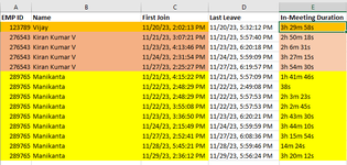
Need total number of days and total duration from the below table data in two cells

For Example For Emp id 289765 he attended from 21 Nov till 29 Nov excluding SAT & SUN the total no of days are 7 hence need no of days as 7 in one cell and on other cell i need total duration of all 7 days he attended that is sum last column which are in HH:MM:SS format
289765​
Manikanta11/21/23, 4:15:22 PM1h 41m 46s
289765​
Manikanta11/22/23, 2:48:29 PM38s
289765​
Manikanta11/22/23, 2:48:29 PM2h 3m 23s
289765​
Manikanta11/22/23, 3:55:08 PM2h 2m 45s
289765​
Manikanta11/23/23, 3:36:50 PM2h 43m 30s
289765​
Manikanta11/24/23, 2:15:49 PM3h 44m 10s
289765​
Manikanta11/27/23, 2:52:41 PM3h 15m 54s
289765​
Manikanta11/28/23, 5:45:21 PM14m 24s
289765​
Manikanta11/29/23, 2:36:12 PM3h 20m 12s
 

Excel Facts

Enter current date or time
Ctrl+: enters current time. Ctrl+; enters current date. Use Ctrl+: Ctrl+; Enter for current date & time.
Are the date and the duration columns date and time just with some formatting or are they text and date and duration should be extracted?
 
Upvote 0
Hi Felix, Objective is for each employee total duration should be extracted in one cell . the date and time are in text format only . I need sum of all the duration like 1h 41m 46s + 38s+2h 3m 23s etc.... into one total duration in one cell
 
Upvote 0
Assuming that dates are in C1:C9 and durations are in D1:D9 then:
for the number of days this formula should work for both version of excel:

Excel Formula:
=SUM((FREQUENCY(DATEVALUE(MID(C1:C9,4,3)&MID(C1:C9,1,3)&MID(C1:C9,7,2)),DATEVALUE(MID(C1:C9,4,3)&MID(C1:C9,1,3)&MID(C1:C9,7,2)))>0)*1)

And for the added duration this formula should work:

Excel Formula:
=SUM(TIME(IFERROR(LEFT(D1:D9,FIND("h",D1:D9)-1),0),IFERROR(IFERROR(MID(D1:D9,FIND("m",D1:D9)-2,2),MID(D1:D9,FIND("m",D1:D9)-1,1)),0),IFERROR(IFERROR(MID(D1:D9,FIND("s",D1:D9)-2,2),MID(D1:D9,FIND("s",D1:D9)-1,1)),0)))

Make sure you press Ctrl+Shift+Enter to enter both formulas. This is needed for the array formulas to work in excel 2016.
For the duration try this cell format: "[h]:mm:ss". If the duration exceeds 24 hours it will show like this example 25:43:12. Else you won't see the hours exceeding 24.
 
Upvote 0
HI Felix, Really appreciate your help and for sharing the formulas. Last one

In the same excel workbook now i have unique EMP ID and EMP Name, Total no of days , Total Duration columns . So by lookup the EMP ID in the other sheet can we sumup all the training duration hours and Total No of days against to each emp in one cell as shown below

EMP IDNameTotal no of daysTotal duration
289765
Manikanta7

Also i am not able to get the total no of days getting error please see the below image

1701962749542.png


1701962809613.png
 
Upvote 0
Try these formulas:
For days:
Excel Formula:
=SUM((FREQUENCY(IFERROR(DATEVALUE(MID(C2:C31,4,3)&MID(C2:C31,1,3)&MID(C2:C31,7,2)),""),IFERROR(DATEVALUE(MID(C2:C31,4,3)&MID(C2:C31,1,3)&MID(C2:C31,7,2)),""))>0)*1)

For duration:
Excel Formula:
=SUM(TIME(IFERROR(LEFT(D2:D31,FIND("h",D2:D31)-1),0),IFERROR(IFERROR(MID(D2:D31,FIND("m",D2:D31)-2,2),MID(D2:D31,FIND("m",D2:D31)-1,1)),0),IFERROR(IFERROR(MID(D2:D31,FIND("s",D2:D31)-2,2),MID(D2:D31,FIND("s",D2:D31)-1,1)),0)))

If you have more data beyond row 31, expand the range to whatever row you need. You can extend it as much as you like, blank cells are ignored.

And remember to enter the formulas with Ctrl+Shift+Enter
 
Upvote 0
HI Felix, Sorry if my question was confusing. I have Main base data sheet ( refer image 1 below ) in one sheet and LOOKUP DATA SHEET in other sheet i have unique employees data ( refer image 2 below ). Now in LOOKUP DATA SHEET i have 4 columns ( EMP ID , EMP Name, Total no of days , Total Duration columns). I need to fetch each employee consolidated Total no of days & Total Duration hours by lookup the EMP ID from the Main data sheet tab)

IMAGE 1:
1701999075293.png


IMAGE2:

1701998940050.png
 

Attachments

  • 1701998979253.png
    1701998979253.png
    46.6 KB · Views: 2
Upvote 0
Try this:

For this example data table:
DayAndDurationFromTextColumns 2 sheets.xlsx
ABCD
1EMP IDNameFirst JoinDuration
2289765Manikanta11/21/23, 4:15:22 PM1h 41m 46s
3289765Manikanta11/22/23, 2:48:29 PM38s
4289765Manikanta11/22/23, 2:48:29 PM2h 3m 23s
5289765Manikanta11/22/23, 3:55:08 PM2h 2m 45s
6289765Manikanta11/23/23, 3:36:50 PM2h 43m 30s
7289765Manikanta11/24/23, 2:15:49 PM3h 44m 10s
8289765Manikanta11/27/23, 2:52:41 PM3h 15m 54s
9289765Manikanta11/28/23, 5:45:21 PM14m 24s
10289765Manikanta11/29/23, 2:36:12 PM3h 20m 12s
1112354Kiran Kumar V10/21/23, 4:15:22 PM2h 2m 45s
1212354Kiran Kumar V10/22/23, 2:48:29 PM2h 43m 30s
1312354Kiran Kumar V10/22/23, 2:48:29 PM3h 44m 10s
1412354Kiran Kumar V10/22/23, 3:55:08 PM3h 15m 54s
15677789Vijay09/01/23, 2:15:49 PM15m 55s
16677789Vijay09/02/23, 1:15:49 PM2h 15m 55s
17677789Vijay09/03/23, 6:05:49 PM1h 35m 5s
Main base data


On the "Lookup Data" sheet:
DayAndDurationFromTextColumns 2 sheets.xlsx
BCD
1NameDaysDuration
2Manikanta719:06:42
3Kiran Kumar V211:46:19
4Vijay34:06:55
Lookup Data
Cell Formulas
RangeFormula
C2:C4C2=SUM((FREQUENCY(IFERROR(IF(DATEVALUE(MID('Main base data'!$C$2:$C$100,4,3)&MID('Main base data'!$C$2:$C$100,1,3)&MID('Main base data'!$C$2:$C$100,7,2))*('Main base data'!$B$2:$B$100=B2)=0,"",DATEVALUE(MID('Main base data'!$C$2:$C$100,4,3)&MID('Main base data'!$C$2:$C$100,1,3)&MID('Main base data'!$C$2:$C$100,7,2))*('Main base data'!$B$2:$B$100=B2)),""),IFERROR(IF(DATEVALUE(MID('Main base data'!$C$2:$C$100,4,3)&MID('Main base data'!$C$2:$C$100,1,3)&MID('Main base data'!$C$2:$C$100,7,2))*('Main base data'!$B$2:$B$100=B2)=0,"",DATEVALUE(MID('Main base data'!$C$2:$C$100,4,3)&MID('Main base data'!$C$2:$C$100,1,3)&MID('Main base data'!$C$2:$C$100,7,2))*('Main base data'!$B$2:$B$100=B2)),""))>0)*1)
D2:D4D2=SUM(TIME(IFERROR(LEFT('Main base data'!$D$2:$D$100,FIND("h",'Main base data'!$D$2:$D$100)-1),0),IFERROR(IFERROR(MID('Main base data'!$D$2:$D$100,FIND("m",'Main base data'!$D$2:$D$100)-2,2),MID('Main base data'!$D$2:$D$100,FIND("m",'Main base data'!$D$2:$D$100)-1,1)),0),IFERROR(IFERROR(MID('Main base data'!$D$2:$D$100,FIND("s",'Main base data'!$D$2:$D$100)-2,2),MID('Main base data'!$D$2:$D$100,FIND("s",'Main base data'!$D$2:$D$100)-1,1)),0))*('Main base data'!$B$2:$B$100=B2))
Press CTRL+SHIFT+ENTER to enter array formulas.


Remember to enter the formulas with Ctrl+Shift+Enter.
Another thing to take into account is that the days formula works if the date is in the format MM/dd/yy. That is if the month or day is less than 10 it will be with a 0 to the left, like 01, 02 and so forth. I you data is not in this format we will have to modify a little the formulas again.
 
Upvote 0
just wondering, what is the date format of your OS? dd/MM/yyyy or MM/dd/yyyy?
 
Upvote 0

Forum statistics

Threads
1,215,069
Messages
6,122,959
Members
449,096
Latest member
Anshu121

We've detected that you are using an adblocker.

We have a great community of people providing Excel help here, but the hosting costs are enormous. You can help keep this site running by allowing ads on MrExcel.com.
Allow Ads at MrExcel

Which adblocker are you using?

Disable AdBlock

Follow these easy steps to disable AdBlock

1)Click on the icon in the browser’s toolbar.
2)Click on the icon in the browser’s toolbar.
2)Click on the "Pause on this site" option.
Go back

Disable AdBlock Plus

Follow these easy steps to disable AdBlock Plus

1)Click on the icon in the browser’s toolbar.
2)Click on the toggle to disable it for "mrexcel.com".
Go back

Disable uBlock Origin

Follow these easy steps to disable uBlock Origin

1)Click on the icon in the browser’s toolbar.
2)Click on the "Power" button.
3)Click on the "Refresh" button.
Go back

Disable uBlock

Follow these easy steps to disable uBlock

1)Click on the icon in the browser’s toolbar.
2)Click on the "Power" button.
3)Click on the "Refresh" button.
Go back
Back
Top