Need formula Index/Match possibly :)

[KDS14589]

I've been trying for days to formulate this with no luck or the solution is so obvious that I can't see it.
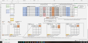
(reference the image) In cells CK9:CK19 I'm trying to match names in cells CA9:CA19 to the names in cells P31:CF41 and return the (min. add) data.
I've hand filled in the data for Jerry to show what I want.
The solution may be a totally different formula than what I've been pursuing, at this point I'm about to start chewing my keyboard...........................

 

[Toadstool]

Hi KDS14589,

Try

=INDEX($P$31:$CH$41,SUMPRODUCT(($P$31:$CF$41=CA19)*ROW($P$31:$CF$41))-ROW($P$31:$CF$41)+1,SUMPRODUCT(($P$31:$CF$41=CA19)*COLUMN($P$31:$CF$41))-COLUMN($P$31:$CF$41)+3)

 

[KDS14589]

=INDEX($P$31:$CH$41,SUMPRODUCT(($P$31:$CF$41=CA19)*ROW($P$31:$CF$41))-ROW($P$31:$CF$41)+1,SUMPRODUCT(($P$31:$CF$41=CA19)*COLUMN($P$31:$CF$41))-COLUMN($P$31:$CF$41)+3)

I tried both with/without CSE but I get a 4 column solution with strange non-corresponding numbers or #VALUE!

 

[Toadstool]

It's difficult to verify the columns in your image but if no name match is found it will give #VALUE.

Here's my test sheet with just the basic test data:

KDS14589.xlsx
	O	P	Q	R	S																		AK	AL	AM	AN	AO																	BF	BG	BH	BI	BJ															BY	BZ	CA	CB	CC	CD	CE	CF	CG	CH	CI	CJ	CK	CL
19																																																																	Jerry										86
20																																																																	David										15
21																																																																	Jeff										258
22																																																																	Sue										7
23																																																																	Ken										774
24																																																																	Angi										15
25																																																																	Deb										21
26
27
28
29
30
31		Sue	2	7																				Angi	3	15																			Jerry	11	86																							David	3	15
32		Deb	6	21																				Lucy	9	45																			Jeff	33	258																							Terry	9	45
33		Laurel	18	63																																									Ken	99	774
34																																													Lynn	297	555
35
36
Sheet1

Cell Formulas
Range	Formula
CK19:CK25	CK19	=INDEX($P$31:$CH$41,SUMPRODUCT(($P$31:$CF$41=CA19)*ROW($P$31:$CF$41))-ROW($P$31:$CF$41)+1,SUMPRODUCT(($P$31:$CF$41=CA19)*COLUMN($P$31:$CF$41))-COLUMN($P$31:$CF$41)+3)
BH34	BH34	=BH33*3

 

[KDS14589]

It's difficult to verify the columns in your image but if no name match is found it will give #VALUE.

Here's my test sheet with just the basic test data:

KDS14589.xlsx
	O	P	Q	R	S																		AK	AL	AM	AN	AO																	BF	BG	BH	BI	BJ															BY	BZ	CA	CB	CC	CD	CE	CF	CG	CH	CI	CJ	CK	CL
19																																																																	Jerry										86
20																																																																	David										15
21																																																																	Jeff										258
22																																																																	Sue										7
23																																																																	Ken										774
24																																																																	Angi										15
25																																																																	Deb										21
26
27
28
29
30
31		Sue	2	7																				Angi	3	15																			Jerry	11	86																							David	3	15
32		Deb	6	21																				Lucy	9	45																			Jeff	33	258																							Terry	9	45
33		Laurel	18	63																																									Ken	99	774
34																																													Lynn	297	555
35
36
Sheet1

Cell Formulas
Range	Formula
CK19:CK25	CK19	=INDEX($P$31:$CH$41,SUMPRODUCT(($P$31:$CF$41=CA19)*ROW($P$31:$CF$41))-ROW($P$31:$CF$41)+1,SUMPRODUCT(($P$31:$CF$41=CA19)*COLUMN($P$31:$CF$41))-COLUMN($P$31:$CF$41)+3)
BH34	BH34	=BH33*3

It's difficult to verify the columns in your image but if no name match is found it will give #VALUE.

Here's my test sheet with just the basic test data:

KDS14589.xlsx
	O	P	Q	R	S																		AK	AL	AM	AN	AO																	BF	BG	BH	BI	BJ															BY	BZ	CA	CB	CC	CD	CE	CF	CG	CH	CI	CJ	CK	CL
19																																																																	Jerry										86
20																																																																	David										15
21																																																																	Jeff										258
22																																																																	Sue										7
23																																																																	Ken										774
24																																																																	Angi										15
25																																																																	Deb										21
26
27
28
29
30
31		Sue	2	7																				Angi	3	15																			Jerry	11	86																							David	3	15
32		Deb	6	21																				Lucy	9	45																			Jeff	33	258																							Terry	9	45
33		Laurel	18	63																																									Ken	99	774
34																																													Lynn	297	555
35
36
Sheet1

Cell Formulas
Range	Formula
CK19:CK25	CK19	=INDEX($P$31:$CH$41,SUMPRODUCT(($P$31:$CF$41=CA19)*ROW($P$31:$CF$41))-ROW($P$31:$CF$41)+1,SUMPRODUCT(($P$31:$CF$41=CA19)*COLUMN($P$31:$CF$41))-COLUMN($P$31:$CF$41)+3)
BH34	BH34	=BH33*3

It's difficult to verify the columns in your image but if no name match is found it will give #VALUE.

Here's my test sheet with just the basic test data:

KDS14589.xlsx
	O	P	Q	R	S																		AK	AL	AM	AN	AO																	BF	BG	BH	BI	BJ															BY	BZ	CA	CB	CC	CD	CE	CF	CG	CH	CI	CJ	CK	CL
19																																																																	Jerry										86
20																																																																	David										15
21																																																																	Jeff										258
22																																																																	Sue										7
23																																																																	Ken										774
24																																																																	Angi										15
25																																																																	Deb										21
26
27
28
29
30
31		Sue	2	7																				Angi	3	15																			Jerry	11	86																							David	3	15
32		Deb	6	21																				Lucy	9	45																			Jeff	33	258																							Terry	9	45
33		Laurel	18	63																																									Ken	99	774
34																																													Lynn	297	555
35
36
Sheet1

Cell Formulas
Range	Formula
CK19:CK25	CK19	=INDEX($P$31:$CH$41,SUMPRODUCT(($P$31:$CF$41=CA19)*ROW($P$31:$CF$41))-ROW($P$31:$CF$41)+1,SUMPRODUCT(($P$31:$CF$41=CA19)*COLUMN($P$31:$CF$41))-COLUMN($P$31:$CF$41)+3)
BH34	BH34	=BH33*3

I'm confused, which is normal for me. I'm trying to get the (min. add) that corresponds to the clients' name from data in the lower 4 charts.

I'm including a link to a shared online file,, this may help mr excel 06.09.21.xlsx

 

[Toadstool]

Ah! Yes, I'd not got the correct cell addresses in a few places. So

=INDEX($P$31:$CN$41,SUMPRODUCT(($P$31:$CF$41=CA9)*ROW($P$31:$CF$41))-ROW($P$31:$CF$41)+1,SUMPRODUCT(($P$31:$CF$41=CA9)*COLUMN($P$31:$CF$41))-COLUMN($P$31:$CF$41)+9)

works for most but not Sue, Deb or Laurel.

I was relying on the "Min Add" columns being 8 to the right of each name (e.g. "David" is in column 84 and the required $188 is in column 92).
The challenge is that the first set (Sue, Deb and Laurel) have names in column 16 and the "Min Add" in column 20. The other sets are 8 columns apart so can you make the first set consistent or do I need a workaround for the first set?

 

[KDS14589]

Ah! Yes, I'd not got the correct cell addresses in a few places. So

=INDEX($P$31:$CN$41,SUMPRODUCT(($P$31:$CF$41=CA9)*ROW($P$31:$CF$41))-ROW($P$31:$CF$41)+1,SUMPRODUCT(($P$31:$CF$41=CA9)*COLUMN($P$31:$CF$41))-COLUMN($P$31:$CF$41)+9)

works for most but not Sue, Deb or Laurel.

I was relying on the "Min Add" columns being 8 to the right of each name (e.g. "David" is in column 84 and the required $188 is in column 92).
The challenge is that the first set (Sue, Deb and Laurel) have names in column 16 and the "Min Add" in column 20. The other sets are 8 columns apart so can you make the first set consistent or do I need a workaround for the first set?

I'm ashamed to say this but I had a 'eureka' moment in this morning shower ?‍ it involves 'nested if statements' based on the individual's balance and using the 4 levels of amounts and the corresponding min. add.

I appreciate your time & knowledge, I guess I was so involved with complex & difficult formulas that I just needed time away from the task to see a simple solution.

Again THANKS

 

[Toadstool]

You're welcome.
I'm not sure I'm following your fix but I see you marked your own post as the solution so I'm guessing you found a workaround which avoids the need for the lookup.

 

[smozgur]

@KDS14589 - Glad to hear you got the solution.

Do you mind posting about your solution? Then it is perfectly fine to mark your post as the solution to help future readers.

 

[KDS14589]

@KDS14589 - Glad to hear you got the solution.

Do you mind posting about your solution? Then it is perfectly fine to mark your post as the solution to help future readers.

I
I would be glad to post it but after I got the solution to work properly, I move it to my secure spreadsheet and moved the info around so now the cells referenced don’t 'jive' with the image and I deleted the spreadsheet I sent

SORRY