Hello, I'm in the process of creating a shared spreadsheet to track how much time a worker who is on light duty due to Worker's Comp injuries should be paid when they have to leave for Dr or PT appointments. The Workers Comp insurance will pay them for that time away from work. The spreadsheet looks like this so far:

I basically have the formulas which are pasted below in the sheet borrowed from another spreadsheet that uses a somewhat similar approach but with only one set of times and for a completely different purpose. The reason why these formulas look so crazy is in large part due to the formatting of the cells in Columns, C, D, and F thru H. These are Custom formatted so that all a person has to do in those cells is type only the numbers and it will add the colons, so typing 100 it puts it as 01:00 and 308 it puts it as 03:08. This was set up like this just to minimize keying and the formulas I was given work with that. Here is a list of what formulas are located where:
Column E:
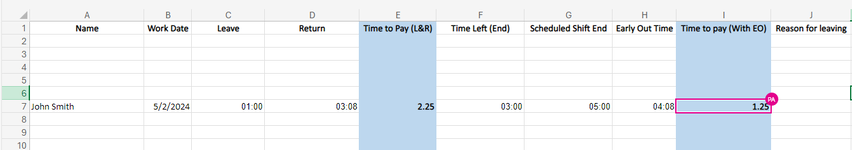
This formula basically subtracts the return time from the leave time to get the total time they are absent. it rounds that to the nearest quarter hour. It also takes into account the possibility of one time being an AM time and the other time being a PM time(The LEN portions of the formula) So with the above screenshot, typing 1000 in C7 for 10:00 would give column E a 4.25 value if the return time 208 (02:08) stays the same.
Column I:
This formula basically does the same as what is in column E but it looks to see if column H has a value. If it does, it will do the calculation from Column F to what is in column H. If there is nothing in H, then it does the calculation from Column F to column G.
What I ultimately want is based on what is illustrated above to have a total column that calculates the totals in Columns E and I. Here's the tricky part though, I can't simply add the two columns together. We reference the screenshot for why. If we look at John Smith's example, he has two sets of time absences, one from the middle of the day and one shortly after that for the end of the day. John's first absence was from 12:00 to 2:08 for one appointment, so 2 hours and 8 minutes which the formula rounds to 2.25 which is correct. John's second absence of time was from 3:00 to 4:08(His shift normally ends at 5:00 but the company offered an early dismissal at 4:08, so his absence time would there would be 1 hour and 8 minutes which the formula rounds to 1.25 which is also correct. If we add both E and I, we would get 3.5 hours. However, if we combine the actual times of absences, we get 3 hours and 16 minutes which rounds to 3.25 hours.
3.25 hours of pay would be the result we are ultimately after, so I am wondering what formula I could use for that. Should it be an additional column, maybe a Grand Total column?
Thank you in advance for the help and let me know if anything needs clarified better.
I basically have the formulas which are pasted below in the sheet borrowed from another spreadsheet that uses a somewhat similar approach but with only one set of times and for a completely different purpose. The reason why these formulas look so crazy is in large part due to the formatting of the cells in Columns, C, D, and F thru H. These are Custom formatted so that all a person has to do in those cells is type only the numbers and it will add the colons, so typing 100 it puts it as 01:00 and 308 it puts it as 03:08. This was set up like this just to minimize keying and the formulas I was given work with that. Here is a list of what formulas are located where:
Column E:
Excel Formula:
=IFERROR(MROUND(IF(OR(AND(LEN(C7)=3,LEN(D7)=3,VALUE(LEFT(C7,1))>VALUE(LEFT(D7,1))),AND(LEN(C7)=4,LEN(D7)=3,VALUE(LEFT(C7,2))>VALUE(LEFT(D7,1))),AND(LEN(C7)=4,LEN(D7)=4,VALUE(LEFT(C7,2))>VALUE(LEFT(D7,2)))),ROUND((TEXT(D7,"00\:00")-TEXT(C7,"00\:00"))*24+(12),2),ROUND((TEXT(D7,"00\:00")-TEXT(C7,"00\:00"))*24,2)),0.25),"")This formula basically subtracts the return time from the leave time to get the total time they are absent. it rounds that to the nearest quarter hour. It also takes into account the possibility of one time being an AM time and the other time being a PM time(The LEN portions of the formula) So with the above screenshot, typing 1000 in C7 for 10:00 would give column E a 4.25 value if the return time 208 (02:08) stays the same.
Column I:
Excel Formula:
=IFERROR(IF(H7="",MROUND(IF(OR(AND(LEN(F7)=3,LEN(G7)=3,VALUE(LEFT(F7,1))>VALUE(LEFT(G7,1))),AND(LEN(F7)=4,LEN(G7)=3,VALUE(LEFT(F7,2))>VALUE(LEFT(G7,1))),AND(LEN(F7)=4,LEN(G7)=4,VALUE(LEFT(F7,2))>VALUE(LEFT(G7,2)))),ROUND((TEXT(G7,"00\:00")-TEXT(F7,"00\:00"))*24+(12),2),ROUND((TEXT(G7,"00\:00")-TEXT(F7,"00\:00"))*24,2)),0.25),MROUND(IF(OR(AND(LEN(F7)=3,LEN(H7)=3,VALUE(LEFT(F7,1))>VALUE(LEFT(H7,1))),AND(LEN(F7)=4,LEN(H7)=3,VALUE(LEFT(F7,2))>VALUE(LEFT(H7,1))),AND(LEN(F7)=4,LEN(H7)=4,VALUE(LEFT(F7,2))>VALUE(LEFT(H7,2)))),ROUND((TEXT(H7,"00\:00")-TEXT(F7,"00\:00"))*24+(12),2),ROUND((TEXT(H7,"00\:00")-TEXT(F7,"00\:00"))*24,2)),0.25)),"")This formula basically does the same as what is in column E but it looks to see if column H has a value. If it does, it will do the calculation from Column F to what is in column H. If there is nothing in H, then it does the calculation from Column F to column G.
What I ultimately want is based on what is illustrated above to have a total column that calculates the totals in Columns E and I. Here's the tricky part though, I can't simply add the two columns together. We reference the screenshot for why. If we look at John Smith's example, he has two sets of time absences, one from the middle of the day and one shortly after that for the end of the day. John's first absence was from 12:00 to 2:08 for one appointment, so 2 hours and 8 minutes which the formula rounds to 2.25 which is correct. John's second absence of time was from 3:00 to 4:08(His shift normally ends at 5:00 but the company offered an early dismissal at 4:08, so his absence time would there would be 1 hour and 8 minutes which the formula rounds to 1.25 which is also correct. If we add both E and I, we would get 3.5 hours. However, if we combine the actual times of absences, we get 3 hours and 16 minutes which rounds to 3.25 hours.
3.25 hours of pay would be the result we are ultimately after, so I am wondering what formula I could use for that. Should it be an additional column, maybe a Grand Total column?
Thank you in advance for the help and let me know if anything needs clarified better.
 I eliminated the MROUND portion from both formulas in E and I and then added a totals column in J. Using the following formula in J


