Need to calculate estimated end date based on rate of spend

[DamianK]

I apologize if I missed threads that discuss this, but I'm trying to calculate the estimated end/depletion date of available money based on current rate of spend.

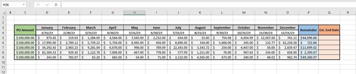
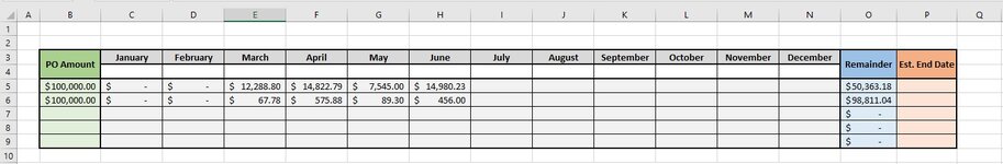
Here's the scenario (per example screenshot):

Column C has a list of PO's.
Column D-O shows amount of money spent against each PO in a given month (again, just an example)
Column P shows the remaining amount of each PO.
Column Q is what I'm trying to figure out.

I need to figure out the formula that calculates the estimated date Column P for each PO will reach zero.

Any help would be much appreciated!

 

[awoohaw]

What are you using as the current rate of spend? The average over the prior 11 months?

 

[awoohaw]

based on average:

Mr Excel Questions2.xlsm
	C	D	E	F	G	H	I	J	K	L	M	N	O	P	Q
1
2	PO AMOUNT	January	February	March	April	May	June	July	August	September	October	November	December	Remainder	Est End Date
3		1/31/2023	2/28/2023	3/31/2023	4/30/2023	5/31/2023	6/30/2023	7/31/2023	8/31/2023	9/30/2023	10/31/2023	11/30/2023	12/31/2023
4	$100,000	$2,251	$3,958	$4,431	$9,551	$6,849	$11,671	$9,378	$6,122	$11,948	$9,685	$11,160	$1,794	$11,202	2/29/2024
5	$100,000	$9,981	$11,648	$9,206	$11,592	$8,099	$3,351	$8,826	$4,231	$7,346	$10,753	$9,105	$7,177	$0
6	$100,000	$11,698	$11,855	$2,020	$10,456	$9,665	$10,790	$8,490	$6,290	$799	$10,252	$9,417	$11,647	$0
7	$100,000	$5,786	$6,982	$11,764	$5,216	$7,625	$10,679	$990	$8,422	$11,821	$4,888	$8,396	$9,779	$7,652	1/31/2024
8	$100,000	$1,353	$2,220	$5,705	$2,361	$1,758	$975	$2,391	$1,409	$9,613	$10,607	$7,059	$2,010	$52,539	2/28/2025
Sheet13

Cell Formulas
Range	Formula
E3:O3	E3	=EOMONTH(D3,1)
P4:P8	P4	=MAX(C4-SUM(D4:O4),0)
Q4:Q7	Q4	=IF(P4=0,"",EOMONTH($O$3,ROUNDUP((P4/ AVERAGEIF(D4:O4,">"&0,D4:O4)),0)))
Q8	Q8	=EOMONTH($O$3,ROUNDUP((P8/ AVERAGEIF(D8:O8,">"&0,D8:O8)),0))

 

[DamianK]

What are you using as the current rate of spend? The average over the prior 11 months?

Great question!

I forgot to mention that the number of months, or the time period the money was spent doesn't matter.

For example, if a PO for 100K was received March 14, 2023, and X amount was spent in April, May and June (or however many months), how would I calculate the approximate date the available funds would reach zero?

As money is spent each month, providing there's still funds remaining, the estimated end date would likely change depending on how much (or little) is spent in each successive month.

 

[awoohaw]

So, in my example above you could have "0.00"amounts beginingin January, or will it be blank until receipts come in?
But you want the average of the months since the PO, right? and Average over those months?
So, what I have done is one scenario of many, but is it correct for that scenario?

 

[awoohaw]

I went back an looked to see if the worksheet formulas I posted early worked with Blanks, Text, or Zeros begining in January, and it seems to work as well Please let me know if you have any errors with it.

 

[DamianK]

So, in my example above you could have "0.00"amounts beginingin January, or will it be blank until receipts come in?
But you want the average of the months since the PO, right? and Average over those months?
So, what I have done is one scenario of many, but is it correct for that scenario?

I've attached a new example. In it, I adjusted the start of the spending to March and ended it in June. It doesn't really matter when the spending begins because it could vary. And though it may matter when creating the formula, knowing the average spend rate doesn't matter to me.

I also limited the number of PO's in the new example to two, and I adjusted the spend rate of the PO in row 5 to show a faster rate than row 6. Based on current spend rate, the money in row 5 will run out long before the money is row 6.

Eventually there will be new spending each month until each PO is empty. But how do I calculate it?

 

[awoohaw]

Okay, this is a new twist. The impression I had was that this all reviewing things after December. I need to look at it more

 

[awoohaw]

how is this:

Mr Excel Questions2.xlsm
	C	D	E	F	G	H	I	J	K	L	M	N	O	P	Q
1
2	PO AMOUNT	January	February	March	April	May	June	July	August	September	October	November	December	Remainder	Est End Date
3		1/31/2023	2/28/2023	3/31/2023	4/30/2023	5/31/2023	6/30/2023	7/31/2023	8/31/2023	9/30/2023	10/31/2023	11/30/2023	12/31/2023
4	$100,000	$2,251	$3,958	$4,431	$9,551	$6,849	$11,671	$9,378	$6,122					$45,789	3/31/2024
5	$100,000				$11,592	$8,099	$3,351	$8,826	$4,231					$63,901	5/31/2024
6	$100,000			$2,020	$10,456	$9,665	$10,790	$8,490	$6,290					$52,289	3/31/2024
7	$100,000	$0	$0	$0	$0	$0	$10,679	$990	$8,422					$79,909	8/31/2024
8	$100,000							$301	$1,409					$98,290	3/31/2033
Rate of Spend Question

Cell Formulas
Range	Formula
E3:O3	E3	=EOMONTH(D3,1)
P4:P8	P4	=MAX(C4-SUM(D4:O4),0)
Q4:Q8	Q4	=EOMONTH( MAX((--(D4:O4>0))*($D$3:$O$3)), ROUNDUP(P4/AVERAGEIF(D4:O4,">"&0,D4:O4),0))

 

[DamianK]

how is this:

Mr Excel Questions2.xlsm
	C	D	E	F	G	H	I	J	K	L	M	N	O	P	Q
1
2	PO AMOUNT	January	February	March	April	May	June	July	August	September	October	November	December	Remainder	Est End Date
3		1/31/2023	2/28/2023	3/31/2023	4/30/2023	5/31/2023	6/30/2023	7/31/2023	8/31/2023	9/30/2023	10/31/2023	11/30/2023	12/31/2023
4	$100,000	$2,251	$3,958	$4,431	$9,551	$6,849	$11,671	$9,378	$6,122					$45,789	3/31/2024
5	$100,000				$11,592	$8,099	$3,351	$8,826	$4,231					$63,901	5/31/2024
6	$100,000			$2,020	$10,456	$9,665	$10,790	$8,490	$6,290					$52,289	3/31/2024
7	$100,000	$0	$0	$0	$0	$0	$10,679	$990	$8,422					$79,909	8/31/2024
8	$100,000							$301	$1,409					$98,290	3/31/2033
Rate of Spend Question

Cell Formulas
Range	Formula
E3:O3	E3	=EOMONTH(D3,1)
P4:P8	P4	=MAX(C4-SUM(D4:O4),0)
Q4:Q8	Q4	=EOMONTH( MAX((--(D4:O4>0))*($D$3:$O$3)), ROUNDUP(P4/AVERAGEIF(D4:O4,">"&0,D4:O4),0))

Thanks!

For column P though, I currently have a formula that auto inputs the remaining money of each PO as money is spent each, so I'm not sure what your formula for that column is for.