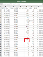
Need to find and highlight values from high column which are greater than 10 times low value but on same expiry date,same strike price,same option typ

[foreveras]

MARKET DATA.xlsx
	A	B	C	D	E	F
1	EXPIRY_Date	STRIKE_PRICE	OPTION_TYPE	HIGH	LOW	DATE
2	29-Dec-22	2150	CE	250	0	01-12-2022
3	30-Dec-22	2200	PE	218.2	0.7	01-12-2022
4	31-Dec-22	3200	PE	190.7	0	01-12-2022
5	01-Jan-23	1200	CE	164.8	1.4	02-12-2022
6	29-Dec-22	2150	PE	141	0	02-12-2022
7	30-Dec-22	2200	PE	119.3	0	02-12-2022
8	30-Dec-22	3200	CE	100.5	0	02-12-2022
9	31-Dec-22	1200	CE	84.5	1.5	02-12-2022
10	01-Jan-23	3200	CE	70.85	0	03-12-2022
11	29-Dec-22	1200	PE	63.75	2	03-12-2022
12	30-Dec-22	2150	PE	48.7	0	03-12-2022
13	31-Dec-22	2200	CE	40.2	0.95	03-12-2022
14	01-Jan-23	2150	PE	33.35	0	03-12-2022
15	29-Dec-22	2200	CE	27.7	3.8	03-12-2022
16	01-Jan-23	3200	PE	23	4.95	03-12-2022
17	29-Dec-22	1200	PE	19.1	4.7	03-12-2022
18	30-Dec-22	3200	CE	15.85	7.25	04-12-2022
19	30-Dec-22	3200	CE	13	6.25	04-12-2022
20	31-Dec-22	1200	PE	2.85	7.45	04-12-2022
21	29-Dec-22	2150	PE	0	9	04-12-2022
22	30-Dec-22	2200	CE	1.9	10.95	04-12-2022
23	31-Dec-22	2150	PE	0	13.4	04-12-2022
24	01-Jan-23	2200	CE	0	16.75	04-12-2022
25	29-Dec-22	2200	PE	0	20.7	04-12-2022
26	30-Dec-22	3200	CE	1.5	26	05-12-2022
27	01-Jan-23	1200	CE	0	32.5	05-12-2022
28	29-Dec-22	3200	PE	2.7	2.95	05-12-2022
29	30-Dec-22	3200	PE	0	0	05-12-2022
30	30-Dec-22	1200	PE	3.15	1.35	05-12-2022
31	31-Dec-22	3200	CE	0	0	05-12-2022
32	01-Jan-23	1200	PE	5.1	0	06-12-2022
33	29-Dec-22	2150	CE	4.95	0	06-12-2022
34	30-Dec-22	2200	PE	6.35	1.55	06-12-2022
35	31-Dec-22	2150	PE	7.25	0	06-12-2022
Sheet2

 

[etaf]

but on same expiry date,same strike price,same option typ​

I was just about to answer the other thread and ask some clarifying questions

can you just outline the criteria for a match please

MAXIFS()

opps pc stuck

 

[foreveras]

In the below image red marked values in HIGH column needed to get highlighted...as its fullfilling the criteria of its 10 times greater than black marked low value..also black marked values expiry date-30 dec 22 ,strike price-3200 and option type - CE all are same to Red marked values and Red marked High values Date also needed to be greater than black marked values date..so same like this criteria need to highlight...I just want to hightlight and find similar to that Red marked values

 

[etaf]

not sur ei fully understand
However, i have added the MAX value based on criteria for that row
see columns G
and the MIN value for the ROW
see columns H

now I have added an IF to compare the ROW to those values

see where i have highlighted
is that the expected result ???

if the value is zero 0 , then 10times is still 0
but i have used if value is 10 or greater

Book5
	A	B	C	D	E	F	G	H	I
1	EXPIRY_Date	STRIKE_PRICE	OPTION_TYPE	HIGH	LOW	DATE	MIN	MAX	possible formula
2	44924	2150	CE	250	0	44896	0	4.95	FALSE
3	44925	2200	PE	218.2	0.7	44896	0	6.35	FALSE
4	44926	3200	PE	190.7	0	44896	0	190.7	TRUE
5	44927	1200	CE	164.8	1.4	44897	1.4	0	TRUE
6	44924	2150	PE	141	0	44897	0	0	FALSE
7	44925	2200	PE	119.3	0	44897	0	6.35	FALSE
8	44925	3200	CE	100.5	0	44897	0	1.5	FALSE
9	44926	1200	CE	84.5	1.5	44897	1.5	84.5	FALSE
10	44927	3200	CE	70.85	0	44898	0	70.85	TRUE
11	44924	1200	PE	63.75	2	44898	2	19.1	TRUE
12	44925	2150	PE	48.7	0	44898	0	48.7	TRUE
13	44926	2200	CE	40.2	0.95	44898	0.95	40.2	FALSE
14	44927	2150	PE	33.35	0	44898	0	33.35	TRUE
15	44924	2200	CE	27.7	3.8	44898	3.8	27.7	TRUE
16	44927	3200	PE	23	4.95	44898	4.95	23	TRUE
17	44924	1200	PE	19.1	4.7	44898	2	19.1	TRUE
18	44925	3200	CE	15.85	7.25	44899	0	1.5	FALSE
19	44925	3200	CE	13	6.25	44899	0	1.5	FALSE
20	44926	1200	PE	2.85	7.45	44899	7.45	2.85	TRUE
21	44924	2150	PE	0	9	44899	0	0	FALSE
22	44925	2200	CE	1.9	10.95	44899	10.95	1.9	TRUE
23	44926	2150	PE	0	13.4	44899	0	0	FALSE
24	44927	2200	CE	0	16.75	44899	16.75	0	TRUE
25	44924	2200	PE	0	20.7	44899	20.7	0	TRUE
26	44925	3200	CE	1.5	26	44900	0	1.5	FALSE
27	44927	1200	CE	0	32.5	44900	1.4	0	TRUE
28	44924	3200	PE	2.7	2.95	44900	2.95	2.7	TRUE
29	44925	3200	PE	0	0	44900	0	0	FALSE
30	44925	1200	PE	3.15	1.35	44900	1.35	3.15	TRUE
31	44926	3200	CE	0	0	44900	0	0	FALSE
32	44927	1200	PE	5.1	0	44901	0	5.1	FALSE
33	44924	2150	CE	4.95	0	44901	0	4.95	FALSE
34	44925	2200	PE	6.35	1.55	44901	0	6.35	FALSE
35	44926	2150	PE	7.25	0	44901	0	0	FALSE
Sheet1

Cell Formulas
Range	Formula
G2:G35	G2	=MINIFS($E$2:$E$35,$A$2:$A$35,A2,$C$2:$C$35,C2,$B$2:$B$35,B2)
H2:H35	H2	=MINIFS($D$2:$D$35,$A$2:$A$35,A2,$C$2:$C$35,C2,$B$2:$B$35,B2)
I2:I35	I2	=IF(G2=0,H2>=10,H2/10<=G2)

Cells with Conditional Formatting
Cell	Condition		Cell Format	Stop If True
A1:I35	Expression	=$I1=TRUE	text	YES