Nested IF, AND Functions Limit Reached. Are there any alternatives?

[stannard3]

Hi,

I am new to Excel. I have been creating a formula combining the IF,AND functions and have just found out that there is a limit to the number of nested formulas.
I still have a lot of criteria to enter so are there any alternatives I can use?

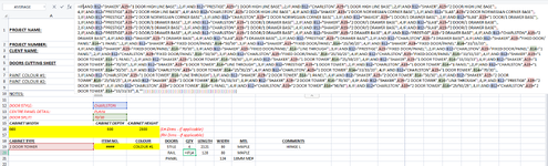
I have attached a screenshot of where I am currently at in a particular cell and seem to have reached a limit. I am new to this so I'm sure there would have been a better way of doing this.

Any help would be greatly appreciated.

Thank you!

 

[etaf]

how many versions are there
group all the results together - so all 2's and 3's
then use a AND() and OR() together

so for 2 you have common things , so a true result only appears once -

like this - from what i can see this is all the 2's

IF( AND( A19="1 line base ", OR( B12 = "shaker", B12="Prestige", B12="chalreston") ) , 2 ,IF ( now group for the 3 , 4 5 6 etc

that would be a nested 8

maybe other ways - but its difficult to see images etc

Note: Images are difficult to see , and also requires that I input all the data myself, which is very time consuming.

A SMALL sample spreadsheet, around 10-20 rows, would help a lot here, with all sensitive data removed, and expected results mocked up and manually entered, with a few notes of explanation.

MrExcel has a tool called “XL2BB” that lets you post samples of your data and will allow us to copy/paste your sample data into our Excel spreadsheets, saving a lot of time.

XL2BB - Excel Range to BBCode

Excel 'mini-sheet' in messages - XL2BB Although experts prefer to read your description and question instead of working in your actual file to solve your problem, there are times that it is difficult to explain an issue without providing actual...

www.mrexcel.com

You can also test to see if it works ok, in the "Test Here" forum.

Test Here

Use this forum to test your signature, learn bbcode, smilies, XL2BB, etc. Threads in this forum are automatically deleted after no replies for seven (7) days

www.mrexcel.com

OR if you cannot get XL2BB to work, or have restrictions on your PC , then put the sample spreadsheet onto a share
I only tend to goto OneDrive, Dropbox or google docs , as I'm never certain of other random share sites and possible virus.
Please make sure you have a representative data sample and also that the data has been desensitised, remember this site is open to anyone with internet access to see - so any sensitive / personal data should be removed

 

[jasonb75]

Another option might be a lookup table. It's not as simple when you have more than 2 sets of criteria to work with but it could be possible.

In order to help you set one up, I would need the following information.

List of options for B12
List of options for A19
List of options for B14

If your attempted formula contains all options (and if you still have it), then copying that and pasting it to the forum will give me all of the info that I need.

It might be a bit harder to set up initially but a lookup table would be easier to maintain than a nested formula if and when any changes are needed.

 

[stannard3]

Another option might be a lookup table. It's not as simple when you have more than 2 sets of criteria to work with but it could be possible.

In order to help you set one up, I would need the following information.

List of options for B12
List of options for A19
List of options for B14

If your attempted formula contains all options (and if you still have it), then copying that and pasting it to the forum will give me all of the info that I need.

It might be a bit harder to set up initially but a lookup table would be easier to maintain than a nested formula if and when any changes are needed.

Thank you for replying! That is a worry I had about the changes required as this document will constantly be updated and evolved.

That sounds great thank you. The formula in the image I posted is about half of the formula I would have needed. Essentially I was working through each Cabinet Type (Cell A19) and creating the criteria needed for each Door Style (Cell B12) and Door Split (Cell B14). I was currently about half way through the Cabinet Types.

See below list of the options for each cell you asked for:

A19 :
1 DOOR HIGH LINE BASE
2 DOOR HIGH LINE BASE
2 DOOR NORWEGIAN CORNER BASE
1 DOOR/1 DRAWER BASE
2 DOOR/1 DRAWER BASE
2 DOOR/2 DRAWER BASE
2 DRAWER BASE
3 DRAWER BASE
5 DRAWER BASE
FIXED DOOR/PANEL
1 DOOR TOWER
2 DOOR TOWER
1 DOOR COUNTER TOP
2 DOOR COUNTER TOP
3 DOOR COUNTER TOP
4 DOOR COUNTER TOP
1 DOOR COUNTER TOP - NBR
2 DOOR COUNTER TOP - NBR
3 DOOR COUNTER TOP - NBR
4 DOOR COUNTER TOP - NBR
1 DOOR WALL
2 DOOR WALL
2 DOOR NORWEGIAN CORNER WALL
1 DOOR TOP BOX
2 DOOR TOP BOX

B12:
SHAKER
SLAB
PRESTIGE
CHARLSTON

B14:
1 PANEL
50/50
25/50/25
33/33/33
70/30
LINE THROUGH

Thanks for your help!

 

[stannard3]

how many versions are there
group all the results together - so all 2's and 3's
then use a AND() and OR() together

so for 2 you have common things , so a true result only appears once -

like this - from what i can see this is all the 2's

IF( AND( A19="1 line base ", OR( B12 = "shaker", B12="Prestige", B12="chalreston") ) , 2 ,IF ( now group for the 3 , 4 5 6 etc

that would be a nested 8

maybe other ways - but its difficult to see images etc

Note: Images are difficult to see , and also requires that I input all the data myself, which is very time consuming.

A SMALL sample spreadsheet, around 10-20 rows, would help a lot here, with all sensitive data removed, and expected results mocked up and manually entered, with a few notes of explanation.

MrExcel has a tool called “XL2BB” that lets you post samples of your data and will allow us to copy/paste your sample data into our Excel spreadsheets, saving a lot of time.

XL2BB - Excel Range to BBCode

Excel 'mini-sheet' in messages - XL2BB Although experts prefer to read your description and question instead of working in your actual file to solve your problem, there are times that it is difficult to explain an issue without providing actual...

www.mrexcel.com

You can also test to see if it works ok, in the "Test Here" forum.

Test Here

Use this forum to test your signature, learn bbcode, smilies, XL2BB, etc. Threads in this forum are automatically deleted after no replies for seven (7) days

www.mrexcel.com

OR if you cannot get XL2BB to work, or have restrictions on your PC , then put the sample spreadsheet onto a share
I only tend to goto OneDrive, Dropbox or google docs , as I'm never certain of other random share sites and possible virus.
Please make sure you have a representative data sample and also that the data has been desensitised, remember this site is open to anyone with internet access to see - so any sensitive / personal data should be removed

Thanks for replying! That makes sense about grouping the criteria by the result I need rather than the criteria. I will give that if the lookup table does not work.

Thank you!

 

[etaf]

the lookup table is the way to go and could even just use a countifs() , so A19 seems to be the number determinator - and so the others B12 and B14 does not change the number at all

then maybe a lookup just for A19 might work - I'll leave for now with jasonb75
but happy to make up something for you , if no reply

And it appears the number only goes up to 5 - yet you had the number 8 in the sample, i seem to remember "door tower" - is that the complete list

 

[jasonb75]

I'm a bit pressed for time today so I've been putting something together quickly while I was waiting on your reply. I think that I've managed to get everything in from the formula in your screen capture but my eyes are starting to spin a bit reading it so anything is possible.

I've added the table to the side of the sheet for reference, but to keep things tidy it is often preferred to have the table on another sheet (which can be hidden if desired).

The results for the combinations go in the yellow part of the table, for combinations that don't exist, you can leave it blank (the formula will return 0).
It consists of 4 columns, 1 for each possible entry in B12

Column H contains the options for A19, followed by the paired options for A19 and B14 spanning columns G and H (the visual in the sheet will probably make more sense than my attempt to explain).

Given that each combination in the table will be unique, we can use a sum function to pull the required result from the cell (this is a lot easier to do with numbers than it is with text).

Moving on to the formula, the INDEX(MATCH( part of it identifies the correct column of results based on the selection in B12. Then SUMIFS uses the selections in A19 and B14 to find the value in the correct row.

I'm going to be away from the forum (or at least away from my laptop) in about an hour and won't be back to it for a few days. @etaf, would you be able to assist with any follow up questions please? I can respond to basics from my phone, but code and formulas are near impossible.

Stannard3.xlsx
	A	B	C	D	E	F	G	H	I	J	K	L
1									Shaker	Prestige	Charlston	Slab
2								1 Door High Line Base	2	2	2
3								2 Door High Line Base	4	4	4
4								2 Door Norwegian Corner Base	3	3	3
5								1 Door/1 Drawer Base
6								2 Door/1 Drawer Base
7								2 Door/2 Drawer Base
8								2 Drawer Base
9								3 Drawer Base
10							1 Panel	Fixed Door/Panel
11							50/50	Fixed Door/Panel
12		Charlston					25/50/25	Fixed Door/Panel
13							33/33/33	Fixed Door/Panel
14		70/30					70/30	Fixed Door/Panel
15							Line Through	Fixed Door/Panel
16							1 Panel	1 Door Tower
17							50/50	1 Door Tower
18							25/50/25	1 Door Tower
19	2 Door Tower			Result >>	12345		33/33/33	1 Door Tower
20							70/30	1 Door Tower
21							Line Through	1 Door Tower
22							1 Panel	2 Door Tower
23							50/50	2 Door Tower
24							25/50/25	2 Door Tower
25							33/33/33	2 Door Tower
26							70/30	2 Door Tower			12345
27							Line Through	2 Door Tower
Sheet1

Cell Formulas
Range	Formula
E19	E19	=SUMIFS(INDEX($I$2:$L$27,0,MATCH(B12,$I$1:$L$1,0)),$H$2:$H$27,A19,$G$2:$G$27,B14&"")

 

[etaf]

would you be able to assist with any follow up questions please?

of course , I think this may just be a simple lookup from A19 - but await the OP reply to my questions in last post

 

[stannard3]

I'm a bit pressed for time today so I've been putting something together quickly while I was waiting on your reply. I think that I've managed to get everything in from the formula in your screen capture but my eyes are starting to spin a bit reading it so anything is possible.

I've added the table to the side of the sheet for reference, but to keep things tidy it is often preferred to have the table on another sheet (which can be hidden if desired).

The results for the combinations go in the yellow part of the table, for combinations that don't exist, you can leave it blank (the formula will return 0).
It consists of 4 columns, 1 for each possible entry in B12

Column H contains the options for A19, followed by the paired options for A19 and B14 spanning columns G and H (the visual in the sheet will probably make more sense than my attempt to explain).

Given that each combination in the table will be unique, we can use a sum function to pull the required result from the cell (this is a lot easier to do with numbers than it is with text).

Moving on to the formula, the INDEX(MATCH( part of it identifies the correct column of results based on the selection in B12. Then SUMIFS uses the selections in A19 and B14 to find the value in the correct row.

I'm going to be away from the forum (or at least away from my laptop) in about an hour and won't be back to it for a few days. @etaf, would you be able to assist with any follow up questions please? I can respond to basics from my phone, but code and formulas are near impossible.

Stannard3.xlsx
	A	B	C	D	E	F	G	H	I	J	K	L
1									Shaker	Prestige	Charlston	Slab
2								1 Door High Line Base	2	2	2
3								2 Door High Line Base	4	4	4
4								2 Door Norwegian Corner Base	3	3	3
5								1 Door/1 Drawer Base
6								2 Door/1 Drawer Base
7								2 Door/2 Drawer Base
8								2 Drawer Base
9								3 Drawer Base
10							1 Panel	Fixed Door/Panel
11							50/50	Fixed Door/Panel
12		Charlston					25/50/25	Fixed Door/Panel
13							33/33/33	Fixed Door/Panel
14		70/30					70/30	Fixed Door/Panel
15							Line Through	Fixed Door/Panel
16							1 Panel	1 Door Tower
17							50/50	1 Door Tower
18							25/50/25	1 Door Tower
19	2 Door Tower			Result >>	12345		33/33/33	1 Door Tower
20							70/30	1 Door Tower
21							Line Through	1 Door Tower
22							1 Panel	2 Door Tower
23							50/50	2 Door Tower
24							25/50/25	2 Door Tower
25							33/33/33	2 Door Tower
26							70/30	2 Door Tower			12345
27							Line Through	2 Door Tower
Sheet1

Cell Formulas
Range	Formula
E19	E19	=SUMIFS(INDEX($I$2:$L$27,0,MATCH(B12,$I$1:$L$1,0)),$H$2:$H$27,A19,$G$2:$G$27,B14&"")

Hi Both!,

Thank you so much! That looks like it is going to work. I will get a chance to test this properly later this afternoon and let you know how it comes out.
Presumably I can use this for other cells where I need to do a particular calculation depending on the cabinet type a d door style etc. I guess this would also work by changing the yellow boxes to the relevant formula.

I am also going to be away until later this afternoon but Thanks again @etaf and @jasonb75

 

[etaf]

I will get a chance to test this properly later this afternoon and let you know how it comes out.

OK