Pricing cluster graph

[imessner]

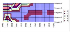
I'm trying to figure out a nice way to do a pricing cluster graph in excel. I've tried using cluster graphs, but if you have 2 or more items at the same price you only get one data point, It won't show a larger data point or have any way of showing multiple products for that price point. This is something that comes up all the time & I have an very unattractive way of graphing these (not actually in a really graph, I make a chart and fill in cells with different colors to represent companys/prices and use several lines to represent multiple pricing at one price level)


<TABLE style="WIDTH: 432pt; BORDER-COLLAPSE: collapse" cellSpacing=0 cellPadding=0 width=576 border=0 x:str><COLGROUP><COL style="WIDTH: 96pt; mso-width-source: userset; mso-width-alt: 4681" width=128><COL style="WIDTH: 48pt" span=7 width=64><TBODY><TR style="HEIGHT: 12.75pt" height=17><TD style="BORDER-RIGHT: #d4d0c8; BORDER-TOP: #d4d0c8; BORDER-LEFT: #d4d0c8; WIDTH: 96pt; BORDER-BOTTOM: #d4d0c8; HEIGHT: 12.75pt; BACKGROUND-COLOR: transparent" width=128 height=17>Water bottle pricing</TD><TD style="BORDER-RIGHT: #d4d0c8; BORDER-TOP: #d4d0c8; BORDER-LEFT: #d4d0c8; WIDTH: 48pt; BORDER-BOTTOM: #d4d0c8; BACKGROUND-COLOR: transparent" width=64></TD><TD style="BORDER-RIGHT: #d4d0c8; BORDER-TOP: #d4d0c8; BORDER-LEFT: #d4d0c8; WIDTH: 48pt; BORDER-BOTTOM: #d4d0c8; BACKGROUND-COLOR: transparent" width=64></TD><TD style="BORDER-RIGHT: #d4d0c8; BORDER-TOP: #d4d0c8; BORDER-LEFT: #d4d0c8; WIDTH: 48pt; BORDER-BOTTOM: #d4d0c8; BACKGROUND-COLOR: transparent" width=64></TD><TD style="BORDER-RIGHT: #d4d0c8; BORDER-TOP: #d4d0c8; BORDER-LEFT: #d4d0c8; WIDTH: 48pt; BORDER-BOTTOM: #d4d0c8; BACKGROUND-COLOR: transparent" width=64></TD><TD style="BORDER-RIGHT: #d4d0c8; BORDER-TOP: #d4d0c8; BORDER-LEFT: #d4d0c8; WIDTH: 48pt; BORDER-BOTTOM: #d4d0c8; BACKGROUND-COLOR: transparent" width=64></TD><TD style="BORDER-RIGHT: #d4d0c8; BORDER-TOP: #d4d0c8; BORDER-LEFT: #d4d0c8; WIDTH: 48pt; BORDER-BOTTOM: #d4d0c8; BACKGROUND-COLOR: transparent" width=64></TD><TD style="BORDER-RIGHT: #d4d0c8; BORDER-TOP: #d4d0c8; BORDER-LEFT: #d4d0c8; WIDTH: 48pt; BORDER-BOTTOM: #d4d0c8; BACKGROUND-COLOR: transparent" width=64></TD></TR><TR style="HEIGHT: 12.75pt" height=17><TD style="BORDER-RIGHT: #d4d0c8; BORDER-TOP: #d4d0c8; BORDER-LEFT: #d4d0c8; BORDER-BOTTOM: #d4d0c8; HEIGHT: 12.75pt; BACKGROUND-COLOR: transparent" height=17></TD><TD style="BORDER-RIGHT: #d4d0c8; BORDER-TOP: #d4d0c8; BORDER-LEFT: #d4d0c8; BORDER-BOTTOM: #d4d0c8; BACKGROUND-COLOR: transparent"></TD><TD style="BORDER-RIGHT: #d4d0c8; BORDER-TOP: #d4d0c8; BORDER-LEFT: #d4d0c8; BORDER-BOTTOM: #d4d0c8; BACKGROUND-COLOR: transparent"></TD><TD style="BORDER-RIGHT: #d4d0c8; BORDER-TOP: #d4d0c8; BORDER-LEFT: #d4d0c8; BORDER-BOTTOM: #d4d0c8; BACKGROUND-COLOR: transparent"></TD><TD style="BORDER-RIGHT: #d4d0c8; BORDER-TOP: #d4d0c8; BORDER-LEFT: #d4d0c8; BORDER-BOTTOM: #d4d0c8; BACKGROUND-COLOR: transparent"></TD><TD style="BORDER-RIGHT: #d4d0c8; BORDER-TOP: #d4d0c8; BORDER-LEFT: #d4d0c8; BORDER-BOTTOM: #d4d0c8; BACKGROUND-COLOR: transparent"></TD><TD style="BORDER-RIGHT: #d4d0c8; BORDER-TOP: #d4d0c8; BORDER-LEFT: #d4d0c8; BORDER-BOTTOM: #d4d0c8; BACKGROUND-COLOR: transparent"></TD><TD style="BORDER-RIGHT: #d4d0c8; BORDER-TOP: #d4d0c8; BORDER-LEFT: #d4d0c8; BORDER-BOTTOM: #d4d0c8; BACKGROUND-COLOR: transparent"></TD></TR><TR style="HEIGHT: 12.75pt" height=17><TD style="BORDER-RIGHT: #d4d0c8; BORDER-TOP: #d4d0c8; BORDER-LEFT: #d4d0c8; BORDER-BOTTOM: #d4d0c8; HEIGHT: 12.75pt; BACKGROUND-COLOR: transparent" height=17>Company Name</TD><TD style="BORDER-RIGHT: #d4d0c8; BORDER-TOP: #d4d0c8; BORDER-LEFT: #d4d0c8; BORDER-BOTTOM: #d4d0c8; BACKGROUND-COLOR: transparent"></TD><TD style="BORDER-RIGHT: #d4d0c8; BORDER-TOP: #d4d0c8; BORDER-LEFT: #d4d0c8; BORDER-BOTTOM: #d4d0c8; BACKGROUND-COLOR: transparent"></TD><TD style="BORDER-RIGHT: #d4d0c8; BORDER-TOP: #d4d0c8; BORDER-LEFT: #d4d0c8; BORDER-BOTTOM: #d4d0c8; BACKGROUND-COLOR: transparent"></TD><TD style="BORDER-RIGHT: #d4d0c8; BORDER-TOP: #d4d0c8; BORDER-LEFT: #d4d0c8; BORDER-BOTTOM: #d4d0c8; BACKGROUND-COLOR: transparent"></TD><TD style="BORDER-RIGHT: #d4d0c8; BORDER-TOP: #d4d0c8; BORDER-LEFT: #d4d0c8; BORDER-BOTTOM: #d4d0c8; BACKGROUND-COLOR: transparent"></TD><TD style="BORDER-RIGHT: #d4d0c8; BORDER-TOP: #d4d0c8; BORDER-LEFT: #d4d0c8; BORDER-BOTTOM: #d4d0c8; BACKGROUND-COLOR: transparent"></TD><TD style="BORDER-RIGHT: #d4d0c8; BORDER-TOP: #d4d0c8; BORDER-LEFT: #d4d0c8; BORDER-BOTTOM: #d4d0c8; BACKGROUND-COLOR: transparent"></TD></TR><TR style="HEIGHT: 12.75pt" height=17><TD style="BORDER-RIGHT: #d4d0c8; BORDER-TOP: #d4d0c8; BORDER-LEFT: #d4d0c8; BORDER-BOTTOM: #d4d0c8; HEIGHT: 12.75pt; BACKGROUND-COLOR: transparent" height=17>Company 1</TD><TD class=xl24 style="BORDER-RIGHT: #d4d0c8; BORDER-TOP: #d4d0c8; BORDER-LEFT: #d4d0c8; BORDER-BOTTOM: #d4d0c8; BACKGROUND-COLOR: transparent" x:num="4.5"> $ 4.50 </TD><TD class=xl24 style="BORDER-RIGHT: #d4d0c8; BORDER-TOP: #d4d0c8; BORDER-LEFT: #d4d0c8; BORDER-BOTTOM: #d4d0c8; BACKGROUND-COLOR: transparent" x:num="5.25"> $ 5.25 </TD><TD class=xl24 style="BORDER-RIGHT: #d4d0c8; BORDER-TOP: #d4d0c8; BORDER-LEFT: #d4d0c8; BORDER-BOTTOM: #d4d0c8; BACKGROUND-COLOR: transparent" x:num="5.75"> $ 5.75 </TD><TD class=xl24 style="BORDER-RIGHT: #d4d0c8; BORDER-TOP: #d4d0c8; BORDER-LEFT: #d4d0c8; BORDER-BOTTOM: #d4d0c8; BACKGROUND-COLOR: transparent"></TD><TD class=xl24 style="BORDER-RIGHT: #d4d0c8; BORDER-TOP: #d4d0c8; BORDER-LEFT: #d4d0c8; BORDER-BOTTOM: #d4d0c8; BACKGROUND-COLOR: transparent"></TD><TD class=xl24 style="BORDER-RIGHT: #d4d0c8; BORDER-TOP: #d4d0c8; BORDER-LEFT: #d4d0c8; BORDER-BOTTOM: #d4d0c8; BACKGROUND-COLOR: transparent"></TD><TD style="BORDER-RIGHT: #d4d0c8; BORDER-TOP: #d4d0c8; BORDER-LEFT: #d4d0c8; BORDER-BOTTOM: #d4d0c8; BACKGROUND-COLOR: transparent"></TD></TR><TR style="HEIGHT: 12.75pt" height=17><TD style="BORDER-RIGHT: #d4d0c8; BORDER-TOP: #d4d0c8; BORDER-LEFT: #d4d0c8; BORDER-BOTTOM: #d4d0c8; HEIGHT: 12.75pt; BACKGROUND-COLOR: transparent" height=17>Company 2</TD><TD class=xl24 style="BORDER-RIGHT: #d4d0c8; BORDER-TOP: #d4d0c8; BORDER-LEFT: #d4d0c8; BORDER-BOTTOM: #d4d0c8; BACKGROUND-COLOR: transparent" x:num="5"> $ 5.00 </TD><TD class=xl24 style="BORDER-RIGHT: #d4d0c8; BORDER-TOP: #d4d0c8; BORDER-LEFT: #d4d0c8; BORDER-BOTTOM: #d4d0c8; BACKGROUND-COLOR: transparent" x:num="5"> $ 5.00 </TD><TD class=xl24 style="BORDER-RIGHT: #d4d0c8; BORDER-TOP: #d4d0c8; BORDER-LEFT: #d4d0c8; BORDER-BOTTOM: #d4d0c8; BACKGROUND-COLOR: transparent" x:num="5"> $ 5.00 </TD><TD class=xl24 style="BORDER-RIGHT: #d4d0c8; BORDER-TOP: #d4d0c8; BORDER-LEFT: #d4d0c8; BORDER-BOTTOM: #d4d0c8; BACKGROUND-COLOR: transparent" x:num="7"> $ 7.00 </TD><TD class=xl24 style="BORDER-RIGHT: #d4d0c8; BORDER-TOP: #d4d0c8; BORDER-LEFT: #d4d0c8; BORDER-BOTTOM: #d4d0c8; BACKGROUND-COLOR: transparent"></TD><TD class=xl24 style="BORDER-RIGHT: #d4d0c8; BORDER-TOP: #d4d0c8; BORDER-LEFT: #d4d0c8; BORDER-BOTTOM: #d4d0c8; BACKGROUND-COLOR: transparent"></TD><TD style="BORDER-RIGHT: #d4d0c8; BORDER-TOP: #d4d0c8; BORDER-LEFT: #d4d0c8; BORDER-BOTTOM: #d4d0c8; BACKGROUND-COLOR: transparent"></TD></TR><TR style="HEIGHT: 12.75pt" height=17><TD style="BORDER-RIGHT: #d4d0c8; BORDER-TOP: #d4d0c8; BORDER-LEFT: #d4d0c8; BORDER-BOTTOM: #d4d0c8; HEIGHT: 12.75pt; BACKGROUND-COLOR: transparent" height=17>Company 3</TD><TD class=xl24 style="BORDER-RIGHT: #d4d0c8; BORDER-TOP: #d4d0c8; BORDER-LEFT: #d4d0c8; BORDER-BOTTOM: #d4d0c8; BACKGROUND-COLOR: transparent" x:num="7.5"> $ 7.50 </TD><TD class=xl24 style="BORDER-RIGHT: #d4d0c8; BORDER-TOP: #d4d0c8; BORDER-LEFT: #d4d0c8; BORDER-BOTTOM: #d4d0c8; BACKGROUND-COLOR: transparent" x:num="8"> $ 8.00 </TD><TD class=xl24 style="BORDER-RIGHT: #d4d0c8; BORDER-TOP: #d4d0c8; BORDER-LEFT: #d4d0c8; BORDER-BOTTOM: #d4d0c8; BACKGROUND-COLOR: transparent" x:num="8.5"> $ 8.50 </TD><TD class=xl24 style="BORDER-RIGHT: #d4d0c8; BORDER-TOP: #d4d0c8; BORDER-LEFT: #d4d0c8; BORDER-BOTTOM: #d4d0c8; BACKGROUND-COLOR: transparent" x:num="9.5"> $ 9.50 </TD><TD class=xl24 style="BORDER-RIGHT: #d4d0c8; BORDER-TOP: #d4d0c8; BORDER-LEFT: #d4d0c8; BORDER-BOTTOM: #d4d0c8; BACKGROUND-COLOR: transparent" x:num="10"> $ 10.00 </TD><TD class=xl24 style="BORDER-RIGHT: #d4d0c8; BORDER-TOP: #d4d0c8; BORDER-LEFT: #d4d0c8; BORDER-BOTTOM: #d4d0c8; BACKGROUND-COLOR: transparent"></TD><TD style="BORDER-RIGHT: #d4d0c8; BORDER-TOP: #d4d0c8; BORDER-LEFT: #d4d0c8; BORDER-BOTTOM: #d4d0c8; BACKGROUND-COLOR: transparent"></TD></TR><TR style="HEIGHT: 12.75pt" height=17><TD style="BORDER-RIGHT: #d4d0c8; BORDER-TOP: #d4d0c8; BORDER-LEFT: #d4d0c8; BORDER-BOTTOM: #d4d0c8; HEIGHT: 12.75pt; BACKGROUND-COLOR: transparent" height=17>Company 4</TD><TD class=xl24 style="BORDER-RIGHT: #d4d0c8; BORDER-TOP: #d4d0c8; BORDER-LEFT: #d4d0c8; BORDER-BOTTOM: #d4d0c8; BACKGROUND-COLOR: transparent" x:num="4.5"> $ 4.50 </TD><TD class=xl24 style="BORDER-RIGHT: #d4d0c8; BORDER-TOP: #d4d0c8; BORDER-LEFT: #d4d0c8; BORDER-BOTTOM: #d4d0c8; BACKGROUND-COLOR: transparent" x:num="4.5"> $ 4.50 </TD><TD class=xl24 style="BORDER-RIGHT: #d4d0c8; BORDER-TOP: #d4d0c8; BORDER-LEFT: #d4d0c8; BORDER-BOTTOM: #d4d0c8; BACKGROUND-COLOR: transparent" x:num="4.75"> $ 4.75 </TD><TD class=xl24 style="BORDER-RIGHT: #d4d0c8; BORDER-TOP: #d4d0c8; BORDER-LEFT: #d4d0c8; BORDER-BOTTOM: #d4d0c8; BACKGROUND-COLOR: transparent" x:num="4.85"> $ 4.85 </TD><TD class=xl24 style="BORDER-RIGHT: #d4d0c8; BORDER-TOP: #d4d0c8; BORDER-LEFT: #d4d0c8; BORDER-BOTTOM: #d4d0c8; BACKGROUND-COLOR: transparent" x:num="5.25"> $ 5.25 </TD><TD class=xl24 style="BORDER-RIGHT: #d4d0c8; BORDER-TOP: #d4d0c8; BORDER-LEFT: #d4d0c8; BORDER-BOTTOM: #d4d0c8; BACKGROUND-COLOR: transparent" x:num="5.75"> $ 5.75 </TD><TD class=xl24 style="BORDER-RIGHT: #d4d0c8; BORDER-TOP: #d4d0c8; BORDER-LEFT: #d4d0c8; BORDER-BOTTOM: #d4d0c8; BACKGROUND-COLOR: transparent" x:num="5.8"> $ 5.80 </TD></TR><TR style="HEIGHT: 12.75pt" height=17><TD style="BORDER-RIGHT: #d4d0c8; BORDER-TOP: #d4d0c8; BORDER-LEFT: #d4d0c8; BORDER-BOTTOM: #d4d0c8; HEIGHT: 12.75pt; BACKGROUND-COLOR: transparent" height=17>Company 5</TD><TD class=xl24 style="BORDER-RIGHT: #d4d0c8; BORDER-TOP: #d4d0c8; BORDER-LEFT: #d4d0c8; BORDER-BOTTOM: #d4d0c8; BACKGROUND-COLOR: transparent" x:num="6"> $ 6.00 </TD><TD class=xl24 style="BORDER-RIGHT: #d4d0c8; BORDER-TOP: #d4d0c8; BORDER-LEFT: #d4d0c8; BORDER-BOTTOM: #d4d0c8; BACKGROUND-COLOR: transparent" x:num="6.25"> $ 6.25 </TD><TD class=xl24 style="BORDER-RIGHT: #d4d0c8; BORDER-TOP: #d4d0c8; BORDER-LEFT: #d4d0c8; BORDER-BOTTOM: #d4d0c8; BACKGROUND-COLOR: transparent" x:num="6.25"> $ 6.25 </TD><TD class=xl24 style="BORDER-RIGHT: #d4d0c8; BORDER-TOP: #d4d0c8; BORDER-LEFT: #d4d0c8; BORDER-BOTTOM: #d4d0c8; BACKGROUND-COLOR: transparent" x:num="7"> $ 7.00 </TD><TD class=xl24 style="BORDER-RIGHT: #d4d0c8; BORDER-TOP: #d4d0c8; BORDER-LEFT: #d4d0c8; BORDER-BOTTOM: #d4d0c8; BACKGROUND-COLOR: transparent" x:num="7"> $ 7.00 </TD><TD class=xl24 style="BORDER-RIGHT: #d4d0c8; BORDER-TOP: #d4d0c8; BORDER-LEFT: #d4d0c8; BORDER-BOTTOM: #d4d0c8; BACKGROUND-COLOR: transparent" x:num="7.5"> $ 7.50 </TD><TD style="BORDER-RIGHT: #d4d0c8; BORDER-TOP: #d4d0c8; BORDER-LEFT: #d4d0c8; BORDER-BOTTOM: #d4d0c8; BACKGROUND-COLOR: transparent"></TD></TR></TBODY></TABLE>

Any hints would be greatly appreciated.

 

[gardnertoo]

Maybe a surface chart, which is basically a three dimensional chart. X axis could represent each company, Y axis ranges of price points, and Z axis the quantity at each X vs Y. Take your existing data and build a new range of cells to count up how many times a given range of prices occurs for each company. I built a sample with your data:

test.txt
	A	B	C	D	E	F	G	H
3	Company Name
4	Company 1	$4.50	$5.25	$5.75
5	Company 2	$5.00	$5.00	$5.00	$7.00
6	Company 3	$7.50	$8.00	$8.50	$9.50	$10.00
7	Company 4	$4.50	$4.50	$4.75	$4.85	$5.25	$5.75	$5.80
8	Company 5	$6.00	$6.25	$6.25	$7.00	$7.00	$7.50
9
10	From:	$4.25	$4.75	$5.25	$5.75	$6.25	$6.75	$7.25
11	To:	$4.75	$5.25	$5.75	$6.25	$6.75	$7.25	$7.75
12	Center:	$4.50	$5.00	$5.50	$6.00	$6.50	$7.00	$7.50
13	Company 1	1	1	2	1	0	0	0
14	Company 2	0	3	0	0	0	1	0
15	Company 3	0	0	0	0	0	0	1
16	Company 4	3	3	2	2	0	0	0
17	Company 5	0	0	0	3	2	2	1
test

Then graph it in a surface chart. You get better display in a two dimensional chart, but to manipulate the scale of the Z axis you have to be in three dimensions. With more data the effect is better, but you get the idea: