Problems getting 5 functions that work individually to work as one.

[fees4steez]

I am using Excel 2016 on Windows 10. This is also my first post, so if I need to provide more info or change something please let me know!

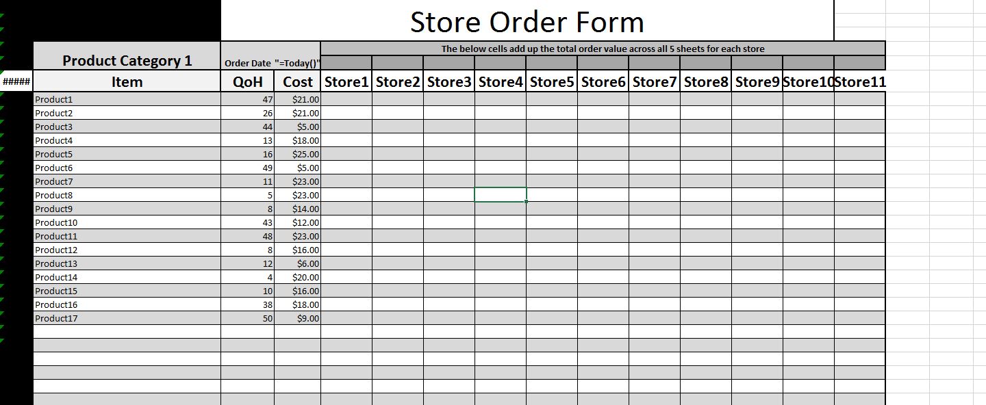
I am building a new order form for our company, and am running into errors. On 5 different sheets are different product categories. Next to those products are a column for each location to input quantity. I am trying to build a formula that will take all the values in those columns and paste it into a cell on the Order form (which would be on the 6th sheet), with a formula to populate the name of the product and cost as well. The key to this formula is that it cannot have blank lines. When I paste each of the five formulas individually, it pulls the correct results. The problem is I cannot get all of them to work together, I either get a #NUM! error or "". These have to be performed as an array formula (Ctrl+Shift+Enter) to work otherwise I get a #VALUE! Error. Through trying IFS, IF, SWITCH, and CHOOSE, I can't get them all to work together. As a test, I populated the first 5 cells in the Array with a unique number to each sheet. The first 5 from the first sheet always populate, but the other ones are either #NUM! or "".

Here are the formulas:

=IF(ROWS(Sheet1!$7:7)<=COUNTA(ARRAY1),INDEX(ARRAY1,SMALL(IF(ARRAY1<>"",ROW(ARRAY1)-MIN(ROW(ARRAY1))+1),ROWS(Juice!$7:7))),"")
=IF(ROWS('Sheet2'!$7:7)<=COUNTA(ARRAY2),INDEX(ARRAY2,SMALL(IF(ARRAY2<>"",ROW(ARRAY2)-MIN(ROW(ARRAY2))+1),ROWS('Sheet2'!$7:7))),"")
=IF(ROWS('Sheet3'!$7:7)<=COUNTA(ARRAY3),INDEX(ARRAY3,SMALL(IF(ARRAY3<>"",ROW(ARRAY3)-MIN(ROW(ARRAY3))+1),ROWS('Sheet3'!$7:7))),"")
=IF(ROWS('Sheet4'!$7:7)<=COUNTA(ARRAY4),INDEX(ARRAY4,SMALL(IF(ARRAY4<>"",ROW(ARRAY4)-MIN(ROW(ARRAY4))+1),ROWS('Sheet4'!$7:7))),"")
=IF(ROWS(Sheet5!$7:7)<=COUNTA(ARRAY5),INDEX(ARRAY5,SMALL(IF(ARRAY5<>"",ROW(ARRAY5)-MIN(ROW(ARRAY5))+1),ROWS(Sheet5!$7:7))),"")

The formulas above populate the quantity of the product. When just one of those formulas is pasted into the cell it works.

=IFERROR(OFFSET(IF(ROWS(Sheet1!$7:7)<=COUNTA(ARRAY1),INDEX(ARRAY1,SMALL(IF(ARRAY1<>"",ROW(ARRAY1)-MIN(ROW(ARRAY1))+1),ROWS(Sheet1!$7:7))),""),,-3),"")
=IFERROR(OFFSET(IF(ROWS('Sheet2'!$7:7)<=COUNTA(ARRAY2),INDEX(ARRAY2,SMALL(IF(ARRAY2<>"",ROW(ARRAY2)-MIN(ROW(ARRAY2))+1),ROWS('Sheet2'!$7:7))),""),,-3),"")
=IFERROR(OFFSET(IF(ROWS('Sheet3'!$7:7)<=COUNTA(ARRAY3),INDEX(ARRAY3,SMALL(IF(ARRAY3<>"",ROW(ARRAY3)-MIN(ROW(ARRAY3))+1),ROWS('Sheet3'!$7:7))),""),,-3),"")
=IFERROR(OFFSET(IF(ROWS('Sheet4'!$7:7)<=COUNTA(ARRAY4),INDEX(ARRAY4,SMALL(IF(ARRAY4<>"",ROW(ARRAY4)-MIN(ROW(ARRAY4))+1),ROWS('Sheet4'!$7:7))),""),,-3),"")
=IFERROR(OFFSET(IF(ROWS(Sheet5!$7:7)<=COUNTA(ARRAY5),INDEX(ARRAY5,SMALL(IF(ARRAY5<>"",ROW(ARRAY5)-MIN(ROW(ARRAY5))+1),ROWS(Sheet5!$7:7))),""),,-3),"")

The formulas above populate the product name.

The first line where you can input quantity (no matter which store) is on the 7th row and 5th column of each sheet. When just one of those formulas is pasted into the cell it works.

I appreciate the help!

 

[fees4steez]

UPDATE: I tried the macro again with the right named ranges with the Macro, but I realized I was formatting it wrong in my formula.

"Array1" is the range '$E$7:$E$499' by name. I noticed in the formula you had it as =ordervals(ROWS($A$2:$A2),1), where I was only inputting the "Array1" range on the text. It worked!! Now I just have to repeat this for the other stores, is there a way to put all of these into this same function? Or do I need to create a new macro for each store. This is so awesome, thank you again! I hope one day to be at that level of knowledge with excel and VBA.

 

[fees4steez]

Also, if I wanted to extract additional data (product cost) how would I do that? I tried adding it and got an error. The Product Name is Offset (0,-3) from quantity, and the cost is Offset (0,-1).

If anything though I can just throw all the product names and costs in one column on my raw data page and vlookup

 

[fees4steez]

Another update- I was able to figure out how to extract the cost data as well by adding it in. Would be pretty simple for me to just repeat this whole process for each store, however if they can all be put into one macro that would be awesome!

 

[Eric W]

Wow!

You've definitely made progress, and that's how you'll increase your expertise, by practicing and experimenting.

However, I'm a little hazy on the exact details of where you are. I do get that you want to combine lookups for other stores in the same function. That should be easy enough. Depending on how your sheets are organized, there could be different ways to go about it.

Are the Sheet1-5 the same layout? Can you show a sample of one sheet with the columns identified?

 

[fees4steez]

Thanks! Before really needing to use Excel I didn't know it was this powerful. It is actually pretty fun seeing what works and what doesnt!

Sheets 1-5 (each representing different product categories) have the same layout, just a different number of products for each one. I'm attaching an image as to how they are all layed out. When doing the different macros, I just had to adjust the offset for each store for cost and product name and also uniquely name each formula, but it wouldn't take as much time to extract data if it was all one macro and formula.

 

[fees4steez]

I don't think the image link worked. Heres another. The black column on the left denotes item status using a color based on conditional formatting.

 

[Eric W]

Here's a variant of the UDF that should work for you:

Public Function OrderVals(ByVal OutRow As Long, ByVal Store As Long, ByVal field)
Dim MySheets As Variant, MyVals As Variant, ctr As Long, i As Long, r As Long, LastRow As Long
    Application.Volatile
    MySheets = Array("Sheet1", "Sheet2", "Sheet3", "Sheet4", "Sheet5")
    
    ctr = 0
    
    For i = 0 To UBound(MySheets)
        With Sheets(MySheets(i))
            On Error GoTo NextI:
            LastRow = .Cells(Rows.Count, "B").End(xlUp).Row
            MyVals = .Range(.Cells(1, 1), .Cells(LastRow, Store + 4)).Value
        End With
        On Error GoTo 0
        
        For r = 7 To LastRow
            If MyVals(r, Store + 4) <> "" Then
                ctr = ctr + 1
                If ctr = OutRow Then
                    Select Case field
                        Case 1, "Item"
                            OrderVals = MyVals(r, 2)
                        Case 2, "QoH"
                            OrderVals = MyVals(r, 3)
                        Case 3, "Cost"
                            OrderVals = MyVals(r, 4)
                        Case 4, "Amt"
                            OrderVals = MyVals(r, Store + 4)
                        Case Else
                            OrderVals = "Unknown choice"
                    End Select
                    Exit Function
                End If
            End If
        Next r
NextI:
    Next i
    
    OrderVals = ""
    
End Function

Change the sheet names in red to match your sheet. Other row and column references are also marked in red in case you need to change them. I tweaked it a bit to make it more efficient. To use it, call it like this:

Excel 2012

	A	B	C	D	E	F	G	H	I	J
1		Store1	Item	Cost	Amt		Store3	Item	Cost	Amt
2			Product1-1	1	1			Product1-1	1	4
3			Product3-1	3	22			Product2-1	2	4
4			Product5-1	5	44			Product4-1	4	4
5			Product4-2	4	2			Product6-1	6	5
6			Product5-2	5	33			Product1-2	1	7
7			Product2-3	2	2			Product2-2	2	7
8			Product4-3	4	2.1			Product3-2	3	7
9			Product6-3	6	4			Product4-2	4	7
10			Product1-1	1	1			Product6-2	6	8
11			Product3-1	3	22			Product6-3	6	99
12			Product5-1	5	44			Product1-1	1	4
13			Product1-1	1	1			Product2-1	2	4
14			Product3-1	3	22			Product4-1	4	4
15			Product5-1	5	44			Product6-1	6	5
16								Product1-1	1	4
17								Product2-1	2	4
18								Product4-1	4	4
19								Product6-1	6	5
20

<colgroup><col><col><col><col><col><col><col><col><col><col><col></colgroup><thead>
</thead><tbody>
</tbody>

Sheet6​

Worksheet Formulas Cell Formula C2 =ordervals(ROWS($A$2:$A2),1,C$1) D2 =ordervals(ROWS($A$2:$A2),1,D$1) E2 =ordervals(ROWS($A$2:$A2),1,E$1) H2 =ordervals(ROWS($A$2:$A2),3,"Item") I2 =ordervals(ROWS($A$2:$A2),3,"Cost") J2 =ordervals(ROWS($A$2:$A2),3,"Amt") <thead> </thead><tbody> </tbody>

<tbody>
</tbody>

The calling parameters are row number (like before), then the store number you want to see, then the field you want to see. For Store1, I used the column headings to select the field. For Store3, I just put the name in the function. Depending on how your Order sheet is laid out, you can probably figure out a way to enter the parameters so that you can enter the formula just once, or maybe once per column, then drag it to where you need it.

 

[fees4steez]

So I got the sheet names changed over. Also for clarification, I have a sheet that has an apostrophe in it. Do I reference it in the macro as "Sheet's" OR "Sheet"s"? I have to replace the apostrophe with quotation when referencing them in formulas. Also, I'm not exactly sure what to change the other parameters to? I should have included this on my last post, but this is the order form that I am putting my formulas into, it is on the 6th sheet, with the final sheet in the book being used for raw data. The value column is just a simple calculation of the total value of qty ordered and unit cost (=IFERROR(IF(OR(A6="",B6*C6=0),"",B6*C6),"")).

[/IMG]

 

[Eric W]

In the macro, define the sheets with the products like this:

MySheets = Array("Shee[COLOR=#ff0000]t's[/COLOR]", "Sheet2", "Sheet3", "Sheet4", "Sheet5")

On your order sheet:

A6: =OrderVals(ROWS($A$6:$A6),$B$3,"Item")
B6: =OrderVals(ROWS($A$6:$A6),$B$3,"Amt")
C6: =OrderVals(ROWS($A$6:$A6),$B$3,"Cost")
D6: should be fine with what you have.

Then select A6:D6 and drag them down as far as needed.

 

[fees4steez]

Awesome, will give it a shot. Been really busy over the last couple weeks so I'm just getting back to this but once I get some time I will sit down and get these implemented and let you know how it goes!