Pull data after specific text

[Al99]

Hi All,

I would like some help on trying to figure out how to perform the following:

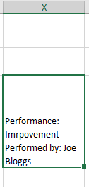
In cell A1 I have the following format of data:
"Performance: Improvement
Performed by: Joe Bloggs"

Essentially, I would like to pull the text just after 'Performance:' part and also pull the text just after 'Performed By:'

This will help me understand if the text is left blank just after 'Performance:' & 'Performed By:'
There is no specific amount of characters that will be after the 'Performance:' & 'Performed By:', this will vary.

Any ideas on how this can be done?

Thanks in advance

 

[GraH]

Maybe like this

Book1
	E	F
3	Performance: Improvement	Improvement
4	Performed by: Joe Bloggs	Joe Bloggs
Sheet1

Cell Formulas
Range	Formula
F3:F4	F3	=MID(E3,FIND(": ",E3)+1,LEN(E3))

 

[etaf]

EDIT
you have an answer above

you should be able to use MID()

Is the bit after Performed by: Joe Bloggs" ALways the last part of the TEXT
for example -
=RIGHT(A2,LEN(A2)-FIND("by:",A2,1)-3)
will extract the Joe Blogs section

 

[Al99]

Hi

Thank you for your updates and help.
So the data will be in the below format, both 'Performance:' and 'Performed by:' will always be there.
However the text after 'Performance:' and 'Performed by:' will always vary
E.G it could change to
'Performance: Decline
Performed by: Joe B'

The aim of this is to understand if the text has been left blank either between performance or performed by.

Thanks

Format of data:

 

[etaf]

=MID(A2,FIND(":",A2,1)+2,FIND("Performed",A2,1)-FIND(":",A2,1)-2)
and
=RIGHT(A2,LEN(A2)-FIND("by:",A2,1)-3)
should extract the data - then if blank how would it look
Performance: Performed by:
Will there just be a SPACE
OR nothing
Performance:Performed by:
You could use an Nested IF () to TEST
BUT would need to know possible permutations

Book1
	A	B	C
1
2	Performance: Improvement Performed by: Joe Bloggs	Joe Bloggs	Improvement
3
Sheet1

Cell Formulas
Range	Formula
B2	B2	=RIGHT(A2,LEN(A2)-FIND("by:",A2,1)-3)
C2	C2	=MID(A2,FIND(":",A2,1)+2,FIND("Performed",A2,1)-FIND(":",A2,1)-2)

 

[Al99]

Thanks again for your help, if blank it would look like this (no spaces after the Performed: or Performed By:

 

[etaf]

So if blank after the Performance: would be performed
If SO then heres a logic test just to see if there are entries after the TAGS Performance & Performed - Could be combined with the other formulas if you wanted to extract the data itself

=IFERROR(IF(AND(FIND("Performed",A3,1)=13,  RIGHT(A1,13)="performed by:"), "Nothing Entered",IF(FIND("Performed",A3,1)=13, "Nothing After Performance",IF(RIGHT(A3,13)="performed by:","Nothing After Performed","data Entered"))),"No Performance OR Performed in text")

Book1
	A	B	C
2	Performance: Improvement Performed by: Joe Bloggs	Joe Bloggs	Improvement
3	Performance:Performed by: Joe Bloggs	Nothing After Performance
4	Performance: Improvement Performed by: Joe Bloggs	data Entered
5	Performance: Improvement Performed by:	Nothing After Performed
6		No Performance OR Performed in text
7		No Performance OR Performed in text
8		No Performance OR Performed in text
Sheet1

Cell Formulas
Range	Formula
C2	C2	=MID(A2,FIND(":",A2,1)+2,FIND("Performed",A2,1)-FIND(":",A2,1)-2)
B2	B2	=RIGHT(A2,LEN(A2)-FIND("by:",A2,1)-3)
B3:B8	B3	=IFERROR(IF(AND(FIND("Performed",A3,1)=13, RIGHT(A1,13)="performed by:"), "Nothing Entered",IF(FIND("Performed",A3,1)=13, "Nothing After Performance",IF(RIGHT(A3,13)="performed by:","Nothing After Performed","data Entered"))),"No Performance OR Performed in text")

 

[riteshkp]

You may also want to try 'Text to columns' in the data menu of excel, using the ":" as as the delimiter.

 

[Peter_SSs]

More possible options.

20 12 13.xlsm
	A	B	C
1		Performance	Performed By
2	Performance: Improvement Performed by: Joe Bloggs	Improvement	Joe Bloggs
3	Performance: Performed by: Joe Bloggs		Joe Bloggs
4	Performance: Improvement Performed by:	Improvement
5	Performance:Performed by:
6	Performance:Increasing Improvement Performed by:JB	Increasing Improvement	JB
Extract Text

Cell Formulas
Range	Formula
B2:B6	B2	=TRIM(MID(A2,13,SEARCH("Performed",A2)-13))
C2:C6	C2	=TRIM(REPLACE(A2,1,FIND(":",A2,13),""))

 

[GraH]

Since I missed the fact both text lines exist in the same cell, maybe this single formula also works
(if only I had let to avoid the repeated filterxlm part...)

Book1
	A	B	C
1	Performance: Improvement Performed by: Joe Bloggs	Improvement	Joe Bloggs
2	Performance: Performed by: Joe Bloggs		Joe Bloggs
3	Performance: Improvement Performed by:	Improvement
4	Performance: Performed by:
5	Performance:Increasing Improvement Performed by:JB	Increasing Improvement	JB
Sheet1

Cell Formulas
Range	Formula
B1:C5	B1	=TRIM(MID(FILTERXML("<text><b>"&SUBSTITUTE($A1,CHAR(10),"</b><b>")&"</b></text>","/text/b["&COLUMNS($B$1:B$1)&"]"),FIND(":",FILTERXML("<text><b>"&SUBSTITUTE($A1,CHAR(10),"</b><b>")&"</b></text>","/text/b["&COLUMNS($B$1:B$1)&"]"))+1,250))