RAG Status Formula

Bidds10

New Member
Joined
Jan 17, 2022
Messages
18
Office Version
  1. 365
Hi All,

This formula is driving me insane. Could anyone help me with the below please? I'm trying to insert a new RAG/SLA status so I don't have to manually change.

RAG =
Before today = "Red"
Is today = "Amber"
Tomorrow = "Yellow"
In future = "White"

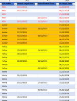
The dates are determined by 3x date columns. Attend Target, Attend Actual and Fix Target.
If 'Fix Target' is before today then "Red", If blank then check if there is a date in 'Attend Target' or 'Attend Actual' If all blank then "White". Else use the closest date.

I hope this makes sense, I've added a picture example of the statuses and dates, Any help would be greatly appreciated.

TIA.


P.S I managed to get this far, but the only status which seems to be correct is "Red" -

=IF(OR(AU5017<TODAY(), AS5017<TODAY()), "Red", IF(OR(ISBLANK(AU5017), ISBLANK(AS5017)), IF(AU5017<TODAY(), "Red", IF(AS5017<TODAY(), "Red")), IF(OR(AU5017=TODAY(), AS5017=TODAY()), "Amber", IF(OR(AU5017=TODAY()+1, AS5017=TODAY()+1), "Yellow", "White"))))
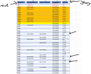
 

Attachments

  • RAG.png
    RAG.png
    33.7 KB · Views: 12

Excel Facts

Format cells as currency
Select range and press Ctrl+Shift+4 to format cells as currency. (Shift 4 is the $ sign).
Maybe this:

Book1
STUVWXYZAAABACADAEAFAGAHAIAJAKALAMANAOAPAQARASATAU
1SLA StatusAttend Target DateAttend Actual DateFix Target Date
212/7/2023Red11/22/202311/22/2023
3Red11/30/202311/30/2023
4Red11/27/2023
5Red11/22/202311/30/2023
6Red11/22/202311/21/202311/29/2023
7Amber12/7/2023
8Amber11/30/202311/23/202312/7/2023
9White12/7/202312/13/2023
10Amber11/30/202311/30/202312/7/2023
11Yellow12/7/202312/8/2023
12White12/7/202312/13/2023
13Yellow12/8/2023
14Yellow10/29/202310/24/202312/8/2023
15White12/8/202312/14/2023
16Yellow12/8/2023
17Yellow10/31/202311/22/202312/8/2023
18Yellow12/8/2023
19Yellow12/5/202312/8/2023
20White12/22/2023
21White12/25/20231/24/2024
22White12/22/2023
23White11/15/202310/17/202312/15/2023
24White
25White9/6/20233/6/2024
26White12/11/2023
27White12/26/20231/25/2024
Sheet1
Cell Formulas
RangeFormula
S2S2=TODAY()
T2:T27T2=IF(AND(AU2="",AT2="",AS2=""),"White",IF(AND(AU2<>"",AU2<TODAY()),"Red",IF(AND(AT2<>"",AU2="",AT2<TODAY()),"Red",IF(AND(AS2<>"",AU2="",AT2="",AS2<TODAY()),"Red",IF(AND(AU2<>"",AU2=TODAY()),"Amber",IF(AND(AT2<>"",AU2="",AT2=TODAY()),"Amber",IF(AND(AS2<>"",AU2="",AT2="",AS2=TODAY()),"Amber",IF(AND(AU2<>"",AU2=TODAY()+1),"Yellow",IF(AND(AT2<>"",AU2="",AT2=TODAY()+1),"Yellow",IF(AND(AS2<>"",AU2="",AT2="",AS2=TODAY()+1),"Yellow","White"))))))))))
 
Upvote 0
Maybe this:

Book1
STUVWXYZAAABACADAEAFAGAHAIAJAKALAMANAOAPAQARASATAU
1SLA StatusAttend Target DateAttend Actual DateFix Target Date
212/7/2023Red11/22/202311/22/2023
3Red11/30/202311/30/2023
4Red11/27/2023
5Red11/22/202311/30/2023
6Red11/22/202311/21/202311/29/2023
7Amber12/7/2023
8Amber11/30/202311/23/202312/7/2023
9White12/7/202312/13/2023
10Amber11/30/202311/30/202312/7/2023
11Yellow12/7/202312/8/2023
12White12/7/202312/13/2023
13Yellow12/8/2023
14Yellow10/29/202310/24/202312/8/2023
15White12/8/202312/14/2023
16Yellow12/8/2023
17Yellow10/31/202311/22/202312/8/2023
18Yellow12/8/2023
19Yellow12/5/202312/8/2023
20White12/22/2023
21White12/25/20231/24/2024
22White12/22/2023
23White11/15/202310/17/202312/15/2023
24White
25White9/6/20233/6/2024
26White12/11/2023
27White12/26/20231/25/2024
Sheet1
Cell Formulas
RangeFormula
S2S2=TODAY()
T2:T27T2=IF(AND(AU2="",AT2="",AS2=""),"White",IF(AND(AU2<>"",AU2<TODAY()),"Red",IF(AND(AT2<>"",AU2="",AT2<TODAY()),"Red",IF(AND(AS2<>"",AU2="",AT2="",AS2<TODAY()),"Red",IF(AND(AU2<>"",AU2=TODAY()),"Amber",IF(AND(AT2<>"",AU2="",AT2=TODAY()),"Amber",IF(AND(AS2<>"",AU2="",AT2="",AS2=TODAY()),"Amber",IF(AND(AU2<>"",AU2=TODAY()+1),"Yellow",IF(AND(AT2<>"",AU2="",AT2=TODAY()+1),"Yellow",IF(AND(AS2<>"",AU2="",AT2="",AS2=TODAY()+1),"Yellow","White"))))))))))

Hello! @dreid1011 Thank you for the fast reply. Really appreciate it! Unfortunately, its still giving me wrong results. Please see attached.
 

Attachments

  • Screenshot.png
    Screenshot.png
    78.3 KB · Views: 6
Upvote 0
If 'Fix Target' is before today then "Red", If blank then check if there is a date in 'Attend Target' or 'Attend Actual' If all blank then "White". Else use the closest date.

What does "closest date" mean? The nearest to today? If so, do you have future dates in there?
 
Upvote 0
What does "closest date" mean? The nearest to today? If so, do you have future dates in there?
Hi @RoryA by closest date I mean closest to today yes, sorry for the confusion. Dates in the future would be classed as "White" status. Thanks.
 
Upvote 0
Maybe this:

Book1
STUVWXYZAAABACADAEAFAGAHAIAJAKALAMANAOAPAQARASATAU
1SLA StatusAttend Target DateAttend Actual DateFix Target Date
212/7/2023Red11/22/202311/22/2023
3Red11/30/202311/30/2023
4Red11/27/2023
5Red11/22/202311/30/2023
6Red11/22/202311/21/202311/29/2023
7Amber12/7/2023
8Amber11/30/202311/23/202312/7/2023
9White12/7/202312/13/2023
10Amber11/30/202311/30/202312/7/2023
11Yellow12/7/202312/8/2023
12White12/7/202312/13/2023
13Yellow12/8/2023
14Yellow10/29/202310/24/202312/8/2023
15White12/8/202312/14/2023
16Yellow12/8/2023
17Yellow10/31/202311/22/202312/8/2023
18Yellow12/8/2023
19Yellow12/5/202312/8/2023
20White12/22/2023
21White12/25/20231/24/2024
22White12/22/2023
23White11/15/202310/17/202312/15/2023
24White
25White9/6/20233/6/2024
26White12/11/2023
27White12/26/20231/25/2024
Sheet1
Cell Formulas
RangeFormula
S2S2=TODAY()
T2:T27T2=IF(AND(AU2="",AT2="",AS2=""),"White",IF(AND(AU2<>"",AU2<TODAY()),"Red",IF(AND(AT2<>"",AU2="",AT2<TODAY()),"Red",IF(AND(AS2<>"",AU2="",AT2="",AS2<TODAY()),"Red",IF(AND(AU2<>"",AU2=TODAY()),"Amber",IF(AND(AT2<>"",AU2="",AT2=TODAY()),"Amber",IF(AND(AS2<>"",AU2="",AT2="",AS2=TODAY()),"Amber",IF(AND(AU2<>"",AU2=TODAY()+1),"Yellow",IF(AND(AT2<>"",AU2="",AT2=TODAY()+1),"Yellow",IF(AND(AS2<>"",AU2="",AT2="",AS2=TODAY()+1),"Yellow","White"))))))))))
Just to confirm, Row 9 on your example should be "red" as there is no Attend Actual Date, only target dates and the earliest one (Attend Actual Target date) is in the past. Hope this makes sense? It's so hard to explain, its driving me mad not being able to figure it out.
 
Upvote 0
Okay, your second image has different dates, so I am not looking at it. I used the original dates again from the first post. Column S below has the new formula results, Column T is manual entry to make sure I understood the rules. See if this is what you want:

Book1 w Stock Room 12-7-2023.xlsm
RSTUVWXYZAAABACADAEAFAGAHAIAJAKALAMANAOAPAQARASATAU
112/9/202312/8/2023SLA StatusAttend Target DateAttend Actual DateFix Target Date
211/22/2023RedRed11/22/202311/22/2023
311/30/2023RedRed11/30/202311/30/2023
41/0/1900RedRed11/27/2023
511/22/2023RedRed11/22/202311/30/2023
611/22/2023RedRed11/22/202311/21/202311/29/2023
71/0/1900RedRed12/7/2023
811/30/2023RedRed11/30/202311/23/202312/7/2023
912/7/2023WhiteWhite12/7/202312/13/2023
1011/30/2023RedRed11/30/202311/30/202312/7/2023
1112/7/2023AmberAmber12/7/202312/8/2023
1212/7/2023WhiteWhite12/7/202312/13/2023
131/0/1900AmberAmber12/8/2023
1410/29/2023AmberAmber10/29/202310/24/202312/8/2023
1512/8/2023WhiteWhite12/8/202312/14/2023
161/0/1900AmberAmber12/8/2023
1711/22/2023AmberAmber10/31/202311/22/202312/8/2023
181/0/1900YellowYellow12/9/2023
1912/5/2023AmberAmber12/5/202312/8/2023
201/0/1900WhiteWhite12/22/2023
211/0/1900WhiteWhite12/25/20231/24/2024
221/0/1900WhiteWhite12/22/2023
2311/15/2023WhiteWhite11/15/202310/17/202312/15/2023
241/0/1900WhiteWhite
259/6/2023WhiteWhite9/6/20233/6/2024
261/0/1900WhiteWhite12/11/2023
271/0/1900WhiteWhite12/26/20231/25/2024
Sheet1
Cell Formulas
RangeFormula
R1R1=TODAY()+1
S1S1=TODAY()
R2:R27R2=MAXIFS(AS2:AT2,AS2:AT2,"<="&TODAY()+1)
S2:S27S2=LET(nd,MAXIFS(AS2:AT2,AS2:AT2,"<="&TODAY()+1),t,TODAY(),f,t+1,IF(OR(AND(AU2="",AT2="",AS2=""),AU2>f,AND(AU2="",nd>f)),"White",IF(OR(AU2<t,AND(AU2="",nd<t)),"Red",IF(OR(AU2=t,AND(AU2="",nd=t)),"Amber",IF(OR(AU2=f,AND(AU2="",nd=f)),"Yellow","")))))
Cells with Conditional Formatting
CellConditionCell FormatStop If True
T2:AU27Expression=$T2="White"textNO
T2:AU27Expression=$T2="Yellow"textNO
T2:AU27Expression=$T2="Amber"textNO
T2:AU27Expression=$T2="Red"textNO

Hi ya, Thank you for the reply! But no sorry. This is still coming out wrong. :( Please see below.

Your column in the one on the right. The correct one is the one on the left.

1702297326713.png
 
Upvote 0
Can you explain why the row with Fix Target as 17 Dec 23 and Attend Target of 17 Nov 23 should be white not red? Surely Fix target is the closest date to today, and that is in the future.
 
Upvote 0
Can you explain why the row with Fix Target as 17 Dec 23 and Attend Target of 17 Nov 23 should be white not red? Surely Fix target is the closest date to today, and that is in the future.
This one is Red because there is no 'actual attend date' stamp. So the 'attend target' was 17th November and this hasn't been met. that's why its Red :) Hope this makes sense? Really appreciate the help!
 
Upvote 0

Forum statistics

Threads
1,215,094
Messages
6,123,071
Members
449,092
Latest member
ipruravindra

We've detected that you are using an adblocker.

We have a great community of people providing Excel help here, but the hosting costs are enormous. You can help keep this site running by allowing ads on MrExcel.com.
Allow Ads at MrExcel

Which adblocker are you using?

Disable AdBlock

Follow these easy steps to disable AdBlock

1)Click on the icon in the browser’s toolbar.
2)Click on the icon in the browser’s toolbar.
2)Click on the "Pause on this site" option.
Go back

Disable AdBlock Plus

Follow these easy steps to disable AdBlock Plus

1)Click on the icon in the browser’s toolbar.
2)Click on the toggle to disable it for "mrexcel.com".
Go back

Disable uBlock Origin

Follow these easy steps to disable uBlock Origin

1)Click on the icon in the browser’s toolbar.
2)Click on the "Power" button.
3)Click on the "Refresh" button.
Go back

Disable uBlock

Follow these easy steps to disable uBlock

1)Click on the icon in the browser’s toolbar.
2)Click on the "Power" button.
3)Click on the "Refresh" button.
Go back
Back
Top