REPEATBYNUMBER

=REPEATBYNUMBER(range)

range
Required. The range (or table) has the first column as the item name and the last column as the repeat number.

REPEATBYNUMBER takes a range (or table) that has the first column as the item name and the last column as the repeat number then returns a new column of rows with the item names repeated by the required number of times.

smozgur

BatCoder
Builders Club Member
Joined
Feb 28, 2002
Messages
2,553
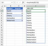
REPEATBYNUMBER function takes a range (or table) that has the first column as the item name and the last column as the repeat number then returns a new column of rows with the item names repeated by the required number of times. (I learned the main idea from Karina Adcock, and used the TAKE function to make it work with a single range/table parameter).

EDIT: This function assumes that each product in the source data exists in the inventory (Repeat >= 1). For an alternative implementation that considers Repeat = 0 please see @Xlambda's RPTBYNR function below.

Excel Formula:
=LAMBDA(data,
    XLOOKUP(
        SEQUENCE(SUM(TAKE(data,,-1))),
        VSTACK(1, SCAN(1,TAKE(data,,-1),LAMBDA(a,b,a+b))),
        VSTACK(TAKE(data,,1),""),
        ,
        -1
    )
)
RepeatByNumber
ABCDEF
1ProductRepeatResult (range param)Result (table param)
2Apple5AppleApple
3Banana4AppleApple
4Cherry2AppleApple
5Strawberry4AppleApple
6AppleApple
7BananaBanana
8BananaBanana
9BananaBanana
10BananaBanana
11CherryCherry
12CherryCherry
13StrawberryStrawberry
14StrawberryStrawberry
15StrawberryStrawberry
16StrawberryStrawberry
Sheet4
Cell Formulas
RangeFormula
D2:D16D2=REPEATBYNUMBER(A2:B5)
F2:F16F2=REPEATBYNUMBER(ProductTable)
Dynamic array formulas.
 
Last edited:
Upvote 1
Hi Suat, really sorry to bother, I am positive you did not read my latest posts under AFLAT thread solving same challenge using same XLOOKUP approach. You would have noticed that the VSTACKs are not needed.
The only difference there, apart of the lack of VSTACKs, is that I have used for running totals MMULT instead of SCAN (that made the formula a formula alternative free of the new functions).
=LET(p,B4:B6,n,C4:C6,r,ROWS(n ),XLOOKUP(SEQUENCE(SUM(n )),MMULT(--(SEQUENCE(r)>=SEQUENCE(,r)),n),p,,1))
Also, if one of the repeating values is 0 , your function REPEATBYNUMBERS delivers wrong results. I know that we can prepare the input array to fit our needs with FILTER or other conditions, but if works for 0's proves that the formulas we use are kind of healthy, algorithm wise.
So, for XLOOKUP approach (with SCAN):
RPTBYNR(a)
Excel Formula:
=LAMBDA(a,
    LET(
        b, TAKE(a, , -1),
        XLOOKUP(SEQUENCE(SUM(b)), SCAN(0, b, LAMBDA(v, i, v + i)), TAKE(a, , 1), , 1)
    )
)
Or an alternative, TOCOL approach:
RPTNTIMES(a)
Excel Formula:
=LAMBDA(a,
    LET(b, TAKE(a, , -1), TOCOL(IF(b >= SEQUENCE(, MAX(b)), TAKE(a, , 1), NA()), 2))
)
repeat product names.xlsx
ABCDEFGHIJKLMN
1if one is 0
2ProductRepeat=REPEATBYNUMBER(A3:B6)ProductRepeat=REPEATBYNUMBER(H3:I6)
3Apple5AppleApple5Apple
4Banana4AppleBanana0Apple
5Cherry2AppleCherry2Apple
6Straberry4AppleStraberry4Apple
7AppleApple
8BananaBanana
9BananaBanana
10BananaStraberry
11BananaStraberry
12CherryStraberry
13CherryStraberry
14Straberry
15Straberry
16Straberry
17Straberry
18
19if one is 0
20ProductRepeat=RPTBYNR(A3:B6)=RPTNTIMES(A3:B6)ProductRepeat=RPTBYNR(H3:I6)=RPTNTIMES(H3:I6)
21Apple5AppleAppleApple5AppleApple
22Banana4AppleAppleBanana0AppleApple
23Cherry2AppleAppleCherry2AppleApple
24Straberry4AppleAppleStraberry4AppleApple
25AppleAppleAppleApple
26BananaBananaCherryCherry
27BananaBananaCherryCherry
28BananaBananaStraberryStraberry
29BananaBananaStraberryStraberry
30CherryCherryStraberryStraberry
31CherryCherryStraberryStraberry
32StraberryStraberry
33StraberryStraberry
34StraberryStraberry
35StraberryStraberry
36
Sheet5
Cell Formulas
RangeFormula
D2,K20,M20,D20,F20,K2D2=FORMULATEXT(D3)
D3:D17,K3:K13D3=REPEATBYNUMBER(A3:B6)
D21:D35,K21:K31D21=RPTBYNR(A3:B6)
F21:F35,M21:M31F21=RPTNTIMES(A3:B6)
Dynamic array formulas.
 
Saw Karina's video. She used the VSTACK's, not you.😉
What triggered me to solve a similar challenge was a comment posted by "EXECUTIVE ENIGNEER" under latest MrExcel YT: Excel IF Contains - 2514 , (where you had also a post.)
We got triggered by different sources. ✌️😉
 
Off topic, a question I wanted to ask you since Excel launched IMAGE function, does it make any sense, or will it be ever possible to integrate IMAGE results on mini sheets using Xl2bb add-in?
What's your opinion on that?
 
I am positive you did not read my latest posts under AFLAT thread solving same challenge using same XLOOKUP approach. You would have noticed that the VSTACKs are not needed.
No, I didn't but now I did, it is beautiful!

And RPTBYNR above is perfect! You know, I am not a perfect function person but a friend asked me for something similar, and I was also curious about how to generate more rows/cols than the source has other than using recursion, and learning the STACK functions made my day. Now I learned another way of that, thank you!
(I only wish that F9 doesn't return #NAME! for the named calculations, it really makes it harder to evaluate the formulas - I have to copy and paste references to analyze the functions.)

Off topic, a question I wanted to ask you since Excel launched IMAGE function, does it make any sense, or will it be ever possible to integrate IMAGE results on mini sheets using Xl2bb add-in?
What's your opinion on that?
I can see at least two potential problems right away with having XL2BB render the URL given to the IMAGE function, and one of them is could be a real pain (dealing with the idea of allowing inner tags in the formula tag). Although I can't promise the implementation, I'll look if I can find a workaround.
 
You're welcome! ✌️🙏
Regarding IMAGE integration, if the cost of integration exceeds the benefits, maybe you don't have to bother spending time on it.
Real benefits, apart from that it will look cool (and nobody has it) are difficult to spot. Anyhow, for images we already have all the fine tools we need, as upload able attachments.
 
I saw the same question from "EXECUTIVE ENIGNEER" on YouTube. It looks like the OP deleted the question, which caused all of the answers to be deleted. My approach to this was a VBA UDF:

VBA Code:
Function Explode(r)
    Dim Answer() As Variant
    CallerRows = r.Rows.Count
    FinalSize = 0
    FinalSize = Application.WorksheetFunction.Sum(r.Columns(2))
    ReDim Answer(1 To FinalSize)
    Ctr = 1
    Debug.Print CallerRows
    For i = 1 To CallerRows
        For j = 1 To r(i, 2).Value
            Answer(Ctr) = r(i, 1).Value
            Ctr = Ctr + 1
        Next j
    Next i
    Explode = Application.Transpose(Answer)
   
End Function
 

Attachments

  • UnusualXL502.png
    UnusualXL502.png
    13.6 KB · Views: 19
I saw the same question from "EXECUTIVE ENIGNEER" on YouTube. It looks like the OP deleted the question, which caused all of the answers to be deleted. My approach to this was a VBA UDF:

VBA Code:
Function Explode(r)
    Dim Answer() As Variant
    CallerRows = r.Rows.Count
    FinalSize = 0
    FinalSize = Application.WorksheetFunction.Sum(r.Columns(2))
    ReDim Answer(1 To FinalSize)
    Ctr = 1
    Debug.Print CallerRows
    For i = 1 To CallerRows
        For j = 1 To r(i, 2).Value
            Answer(Ctr) = r(i, 1).Value
            Ctr = Ctr + 1
        Next j
    Next i
    Explode = Application.Transpose(Answer)
 
End Function
Thanks! VBA will be always my favorite!
 
Power Query version to complete the solution series.

Power Query:
let
    // Load the source table data range
    Source = Excel.CurrentWorkbook(){[Name="ProductTable"]}[Content],

    // Set the column types
    SetTypes = Table.TransformColumnTypes(Source,{{"Product", type text}, {"Repeat", Int64.Type}}),

    // Convert the Repeat column values to many list items by the repeat value
    Repeated = Table.TransformColumns(SetTypes, {"Repeat", each List.Numbers(1,_), type list}),

    // Expand the list items in the converted Repeat column to get the necessary number of repeated rows
    // Note that Product column values are repated for each list item (thát's the whole idea)
    Expanded = Table.ExpandListColumn(Repeated, "Repeat"),

    // Remove items with 0 number of Repeat since those will generate null values (this could be also done at the beginning)
    NullsRemoved = Table.SelectRows(Expanded, each [Repeat] <> null and [Repeat] <> ""),

    // We don't need the Repeat column anymore
    Result = Table.RemoveColumns(NullsRemoved,{"Repeat"})
in
    Result
 
I think this may be more robust.
It works on arrays, returning rows (not just the first column) 'n' times, based on the value in the last column
There is a shortcoming in the current XLOOKUP function in that it cannot return rows of results if the lookup array is a vector (rather than a single value), so I've had to use the REDUCE / VSTACK combo. (I tried MAP (vector, LAMBDA(x, XLOOKUP...), but that didn't work either)

AROWREPEAT: (the final calculation function - DROP - is the fix for the current XLOOKUP function)
Excel Formula:
=LAMBDA(ar,
    LET(
        b, TAKE(ar, , -1),
        c, SEQUENCE(SUM(b)),
        d, SCAN(0, b, LAMBDA(v, i, v + i)),
        DROP(REDUCE(0, c, LAMBDA(a, e, VSTACK(a, XLOOKUP(e, d, DROP(ar,,-1), , 1, 1)))), 1)
    )
)
 
Last edited by a moderator:

Forum statistics

Threads
1,215,357
Messages
6,124,482
Members
449,165
Latest member
ChipDude83

We've detected that you are using an adblocker.

We have a great community of people providing Excel help here, but the hosting costs are enormous. You can help keep this site running by allowing ads on MrExcel.com.
Allow Ads at MrExcel

Which adblocker are you using?

Disable AdBlock

Follow these easy steps to disable AdBlock

1)Click on the icon in the browser’s toolbar.
2)Click on the icon in the browser’s toolbar.
2)Click on the "Pause on this site" option.
Go back

Disable AdBlock Plus

Follow these easy steps to disable AdBlock Plus

1)Click on the icon in the browser’s toolbar.
2)Click on the toggle to disable it for "mrexcel.com".
Go back

Disable uBlock Origin

Follow these easy steps to disable uBlock Origin

1)Click on the icon in the browser’s toolbar.
2)Click on the "Power" button.
3)Click on the "Refresh" button.
Go back

Disable uBlock

Follow these easy steps to disable uBlock

1)Click on the icon in the browser’s toolbar.
2)Click on the "Power" button.
3)Click on the "Refresh" button.
Go back
Back
Top