return a value if a cell is between xx & xx

[juca73]

ill try and keep this simple

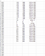
Cell a3 = 598

i have 3 helper columns to produce the range i want displayed based on the value in cell a3

yet i am struggling to get a formula right

so what im asking i want to search column h3-h27 for the range the value in cell a3 falls into then display the result in cell b3

 

[SanjayGMusafir]

Not difficult to solve. Just need 2 things -

~ Use XL2BB tool to post your sample data
~ Update your Account details with Current Excel Version & Platform (Remember to scroll down & Save)

Your Excel Version shows both 365 and 2010 - Both shall have different solution. So update your profile to the latest version you are using.

 

[6StringJazzer]

Your data is a problem because you start by putting the highest number of each range in column F, but starting at -50 you put the lowest number of each range in column F.

The only thing I found that would work is this:

=IFERROR(XLOOKUP(A3,$E$3:$E$13,$G$3:$G$13,,1),XLOOKUP(A3,$F$3:$F$27,$G$3:$G$27,,1))

If you clean your data it is possible to get a cleaner formula.

 

[Peter_SSs]

I agree with @6StringJazzer that columns F:G are in an awful order. If you could arrange them so that column F was always the lowest number in the range then the formula is pretty simple

23 09 10.xlsm
	A	B				F	G	H
1	-598	a				-600	-551	a
2	-150	j				-550	-501	b
3	-4	l				-500	-451	c
4	0	m				-450	-401	d
5	3	n				-400	-351	e
6	211	r				-350	-301	f
7	545	x				-300	-251	g
8						-250	-201	h
9						-200	-151	i
10						-150	-101	j
11						-100	-51	k
12						-50	-1	l
13						0	0	m
14						1	50	n
15						51	100	o
16						101	150	p
17						151	200	q
18						201	250	r
19						251	300	s
20						301	350	t
21						351	400	u
22						401	450	v
23						451	500	w
24						501	550	x
25						551	600	y
Range (2)

Cell Formulas
Range	Formula
B1:B7	B1	=XLOOKUP(A1,F$1:F$25,H$1:H$25,,-1)

If you must keep F:G in the order you have them then you could try this

23 09 10.xlsm
	A	B				F	G	H
1	-598	a				-551	-600	a
2	-150	j				-501	-550	b
3	-4	l				-451	-500	c
4	0	m				-401	-450	d
5	3	n				-351	-400	e
6	211	r				-301	-350	f
7	545	x				-251	-300	g
8						-201	-250	h
9						-151	-200	i
10						-101	-150	j
11						-51	-100	k
12						-50	-1	l
13						0	0	m
14						1	50	n
15						51	100	o
16						101	150	p
17						151	200	q
18						201	250	r
19						251	300	s
20						301	350	t
21						351	400	u
22						401	450	v
23						451	500	w
24						501	550	x
25						551	600	y
Range

Cell Formulas
Range	Formula
B1:B7	B1	=XLOOKUP(A1,IF(A1<-50,F$1:F$25,G$1:G$25),H$1:H$25,,1)