Return a value in a specified column in the same row as a search value

[ShanonExcelQs]

Hi There

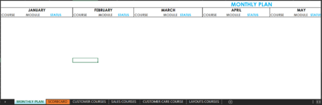
I have a workbook with multiple sheets, and I want to use the first sheet as below "MONTHLY PLAN" to return answers from the other sheets.

In each of the other sheets, I have information regarding modules, like so:

I want to find all the "Modules" that would be for January for example, to show on my first sheet under January. So if we use the above sheet, if in column H the value is "January", I want to see what the corresponding Module is in column B. I would do this for each sheet in the workbook. How would I go about this?

 

[Candyman8019]

Give this a try:
=INDEX('CUSTOMER COURSES'!B2:H$50,MATCH(B$1,'CUSTOMER COURSES'!H2:H$50,0),0)

Assumptions:
- Your month is in Cell B1
- There are 50 rows in your Customer Courses tab...update to however many rows you have.

 

[Toadstool]

Hi ShanonExcelQs,

I have some design comments.

Merged cells are anathema to Excel functions. e.g. Your cell B2 contains "Why promotional products work" and A2 contains "The Promotional Industry - You are here", but B3 contains "The Economic environment - Micro" yet A3 contains nothing and any function retreiving A3 will receive a null string.
You can work around this with a helper column (e.g. create column K as IF(A2<>"",A2,K1) and copy down) but then you need to retrieve Course Names from column K.

Excel Functions can't read the color, font or strikethrough status of a cell. You can use Conditional Formatting to set those things (e.g. if the Status is "Done" then set ETA as strikethrough) but can't read them.

Excel has a limited list of Functions which work as a 3-D reference (i.e. across multiple sheets). You can see that list here: 3-D Functions
You could use INDIRECT and a list of sheet names to do what you want but you'd need some kind of helper column to figure out how many can be listed from each sheet. Messy.

Personally I would use one sheet to contain all Course Types in a new column A. Then the Monthly Plan only need to search that single sheet. Something like this:

ShanonExcelQs.xlsx
	A	B	C	D	E	F	G	H
1	Course Type	Course Name	Module	Source	etc	Status	etc	ETA for Launching / Launched
2	Customer	You are Here	Part 1			Done		09-Sep-21
3	Customer	You are Here	Part 2			Pending		02-Feb-22
4	Customer	You are Here	Part 3			Busy		24-Feb-22
5	Customer	Micro	Part 1			Done		18-Mar-22
6	Customer Care	Cuddle/Coddle	Part 1			Pending		11-Nov-21
7	Customer Care	Cuddle/Coddle	Part 2			Busy		03-Jan-22
8	Layouts	Placement 101	Part 1			Done		25-Dec-21
9	Layouts	Placement 202	Part 2			Pending		16-Jan-22
10	Sales	Oppty Strikes	Part 1			Busy		11-Oct-21
11	Sales	Oppty Strikes	Part 2			Busy		20-Mar-22
12	Sales	Sales 101	Part 1			Done		21-Feb-22
Courses

Cells with Conditional Formatting
Cell	Condition		Cell Format	Stop If True
H2:H999	Expression	=AND(H2<>"",$F$2="Done",H2<TODAY())	text	NO

ShanonExcelQs.xlsx
	A	B	C	D	E	F	G	H	I
1	Monthly Plan
2	Jan-22	Jan-22	Jan-22	Feb-22	Feb-22	Feb-22	Mar-22	Mar-22	Mar-22
3	Course	Module	Status	Course	Module	Status	Course	Module	Status
4	Cuddle/Coddle	Part 2	Busy	You are Here	Part 2	Pending	Micro	Part 1	Done
5	Placement 202	Part 2	Pending	You are Here	Part 3	Busy	Oppty Strikes	Part 2	Busy
6				Sales 101	Part 1	Done
7
MonthlyPlan

Cell Formulas
Range	Formula
D2:I2	D2	=EOMONTH(A2,0)+1
A4:B7	A4	=IFERROR(INDEX(Courses!B$2:B$9999,AGGREGATE(15,6,ROW(Courses!$H$2:$H$9999)-ROW(Courses!$H$1)/((Courses!$H$2:$H$9999>=A$2)*(Courses!$H$2:$H$9999<=EOMONTH(A$2,0))),ROW()-ROW($A$3))),"")
C4:C7	C4	=IFERROR(INDEX(Courses!F$2:F$9999,AGGREGATE(15,6,ROW(Courses!$H$2:$H$9999)-ROW(Courses!$H$1)/((Courses!$H$2:$H$9999>=C$2)*(Courses!$H$2:$H$9999<=EOMONTH(C$2,0))),ROW()-ROW($A$3))),"")
D4:E7	D4	=IFERROR(INDEX(Courses!B$2:B$9999,AGGREGATE(15,6,ROW(Courses!$H$2:$H$9999)-ROW(Courses!$H$1)/((Courses!$H$2:$H$9999>=D$2)*(Courses!$H$2:$H$9999<=EOMONTH(D$2,0))),ROW()-ROW($A$3))),"")
F4:F7	F4	=IFERROR(INDEX(Courses!F$2:F$9999,AGGREGATE(15,6,ROW(Courses!$H$2:$H$9999)-ROW(Courses!$H$1)/((Courses!$H$2:$H$9999>=F$2)*(Courses!$H$2:$H$9999<=EOMONTH(F$2,0))),ROW()-ROW($A$3))),"")
G4:H7	G4	=IFERROR(INDEX(Courses!B$2:B$9999,AGGREGATE(15,6,ROW(Courses!$H$2:$H$9999)-ROW(Courses!$H$1)/((Courses!$H$2:$H$9999>=G$2)*(Courses!$H$2:$H$9999<=EOMONTH(G$2,0))),ROW()-ROW($A$3))),"")
I4:I7	I4	=IFERROR(INDEX(Courses!F$2:F$9999,AGGREGATE(15,6,ROW(Courses!$H$2:$H$9999)-ROW(Courses!$H$1)/((Courses!$H$2:$H$9999>=I$2)*(Courses!$H$2:$H$9999<=EOMONTH(I$2,0))),ROW()-ROW($A$3))),"")

 

[ShanonExcelQs]

Hey Guys

I have updated it to one tab and rearranged a few things, would you be able to help with the formula to get:
The summary of all modules labelled January to be in the Monthly Plan tab. I need the course name, module and the Status. In my courses tab I have no merged cells anymore. I have 225 rows in this tab as well, example image done manually without formula below as how I am trying to get the monthly summary:

AA CONTENT - Internal and External COPY.xlsx
	A	B	C	D	E	F	G	H	I	J	K	L	M	N	O	P	Q	R	S	T	U	V	W	X
1	MONTHLY PLAN
2	JANUARY			FEBRUARY			MARCH			APRIL			MAY			JUNE			JULY			AUGUST
3	COURSE NAME	MODULE	STATUS	COURSE NAME	MODULE	STATUS	COURSE NAME	MODULE	STATUS	COURSE NAME	MODULE	STATUS	COURSE NAME	MODULE	STATUS	COURSE	MODULE	STATUS	COURSE	MODULE	STATUS	COURSE	MODULE	STATUS
MONTHLY PLAN

AA CONTENT - Internal and External COPY.xlsx
	A	B	C	D	E	F	G	H
1	COURSE TYPE	COURSE NAME	MODULE NAME	CONTENT EXPERT	ASSIGNED	STATUS	NOTES	LAUNCH DATE/ETA'S
2	CUSTOMER COURSES	The Promotional Industry - You Are Here	Why promotional products work	Nukiwe	Nukiwe	Done	Launched	Launched
3	CUSTOMER COURSES	The Promotional Industry - You Are Here	The Economic Enviroment - Micro	Nukiwe	Nukiwe	To Create	Create content	February
4	CUSTOMER COURSES	The Promotional Industry - You Are Here	The Economic Enviroment - Macro	Nukiwe	Nukiwe	To Create	Create content	March
5	CUSTOMER COURSES	The Promotional Industry - You Are Here	Managing End User Expectation	Nukiwe	Nukiwe	To Create	Create content	January
6	CUSTOMER COURSES	The Promotional Industry - You Are Here	What's in the bag (Registration Pack)	Nukiwe	Nukiwe	Redo Previous Content	To be Redone	January
7	CUSTOMER COURSES	The Promotional Industry - You Are Here	Introduction to Amrod and the business evolution	Nukiwe	Nukiwe	Redo Previous Content	To be Redone	February
8	CUSTOMER COURSES	The Promotional Industry - You Are Here	Promo Industry in the Post COVID world.	Nukiwe	Nukiwe	To Create	Create content	February
9	CUSTOMER COURSES	The Promotional Industry - You Are Here	Fabrics and Fabrications when selling clothing	Omer		To Create	Create content	February
10	CUSTOMER COURSES	The Promotional Industry - You Are Here	Tips for Success Maximising The Busy Promo Season	Nukiwe	Nukiwe	Done	Content available and edited. Ready to lauch	Launched
11	CUSTOMER COURSES	Sales Tips and Ideas	Capitilize on Collaboration|Understanding your Cients Needs	ASI	ASI	Done	Launched	Launched
12	CUSTOMER COURSES	Sales Tips and Ideas	25 productivity hacks to get things done	ASI	ASI	Done	Launched	Launched
13	CUSTOMER COURSES	Sales Tips and Ideas	Fantastic Follow Ups: Convert Leads Into Sales & Customers Into Fans	ASI	ASI	Done	Launched	Launched
14	CUSTOMER COURSES	Sales Tips and Ideas	Whats Your Bounce Back Plan? 21 Strategies To Implement Today	ASI	ASI	Done	done - ready to launch	Launched
15	CUSTOMER COURSES	Sales Tips and Ideas	Selling to the 21st century	ASI	ASI	Done	Loaded on AA - Not published-awaiting draft mailer from Marketing	Launched
16	CUSTOMER COURSES	Sales Tips and Ideas	Building profitable client relationship	ASI	ASI	Approved - To Launch	Loaded on AA - Not published-mailer to be approved	January
COURSES

Cells with Conditional Formatting
Cell	Condition		Cell Format	Stop If True
C2:H1048576	Expression	=$F2="In Progress"	text	NO
C2:H1048576	Expression	=$F2="Changes Required"/"Approved Script"/"VO Required"	text	NO
C2:H1048576	Expression	=$F2="Approved - to Launch"	text	NO
C2:H1048576	Expression	=$F2="Awaiting Omer Approval"	text	NO
C2:H1048576	Expression	=$F2="Awaiting Feedback"	text	NO
C2:H1048576	Expression	=$F2="To be approved"	text	NO
C2:H1048576	Expression	=$F2="Redo Previous Content"	text	NO
C2:H1048576	Expression	=$F2="To Create"	text	NO
C2:H1048576	Expression	=$F2="Done"	text	NO

Cells with Data Validation
Cell	Allow	Criteria
A2:A16	List	CUSTOMER COURSES; SALES COURSES; CUSTOMER CARE COURSES; LAYOUTS COURSES
F2:F16	List	To Be Approved; To Create; In Progress; Done; Changes Required; Redo Previous Content; Awaiting Feedback; Approved Script; Approved - To Launch; Awaiting Omer Approval; VO Required ; Delayed

 

[Toadstool]

Hi ShanonExcelQs,

I note you didn't change column H to year and month which means you must make sure you don't pick up historical courses. e.g. The August column will pick up any August courses remaining from previous years.

You may want to make column H a dropdown List for month selection. I've added a TRIM to fix your data as some cells, such as H5, had a trailing space and any difference between H and your headings in MonthlyPlan won't find a match.

You said you've removed merged cells but the MonthlyPlan months are still merged so I needed to add the convoluted INDEX($A$2:$X$2,(INT(((COLUMN()-COLUMN($A$3))/3))*3)+1) to match the correct heading month.

I haven't repeated your Courses sheet but here is the MonthlyPlan and you just need to copy the formulae in A4 to X4 down as many rows as will satisfy your maximum courses per month.

ShanonExcelQs-v2.xlsx
	A	B	C	D	E	F	G	H	I	J	K	L	M	N	O	P	Q	R	S	T	U	V	W	X
1	MONTHLY PLAN
2	JANUARY			FEBRUARY			MARCH			APRIL			MAY			JUNE			JULY			AUGUST
3	COURSE NAME	MODULE	STATUS	COURSE NAME	MODULE	STATUS	COURSE NAME	MODULE	STATUS	COURSE NAME	MODULE	STATUS	COURSE NAME	MODULE	STATUS	COURSE NAME	MODULE	STATUS	COURSE NAME	MODULE	STATUS	COURSE NAME	MODULE	STATUS
4	The Promotional Industry - You Are Here	Managing End User Expectation	To Create	The Promotional Industry - You Are Here	The Economic Enviroment - Micro	To Create	The Promotional Industry - You Are Here	The Economic Enviroment - Macro	To Create
5	The Promotional Industry - You Are Here	What's in the bag (Registration Pack)	Redo Previous Content	The Promotional Industry - You Are Here	Introduction to Amrod and the business evolution	Redo Previous Content
6	Sales Tips and Ideas	Building profitable client relationship	Approved - To Launch	The Promotional Industry - You Are Here	Promo Industry in the Post COVID world.	To Create
7				The Promotional Industry - You Are Here	Fabrics and Fabrications when selling clothing	To Create
8
MonthlyPlan

Cell Formulas
Range	Formula
A4:X8	A4	=IFERROR(INDEX(Courses!$B$2:$F$9999,AGGREGATE(15,6,ROW(Courses!$H$2:$H$9999)-ROW(Courses!$H$1)/(TRIM(Courses!$H$2:$H$9999)=INDEX($A$2:$X$2,(INT(((COLUMN()-COLUMN($A$3))/3))*3)+1)),ROW()-ROW($A$3)),CHOOSE(MOD((COLUMN()-COLUMN($A$3)),3)+1,1,2,5)),"")