Returning min value on sum of cells with varying rules

[chr1sj]

Hi, I'm stuck with something in Excel 2019 and am after a solution for the following please:
I have 2 columns of data, A and B.
Columns A and B are populated by other formulae results.
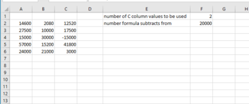
Column E describes the cells in column F in this example.
Cell F1 is manually populated.
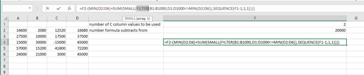
Cell F2 is populated by a formula.
The amount of rows in columns A and B will change as new data is entered.

I need the formula to solve with the following rules:
Exactly one cell from column A must be used.
The cell adjacent to that used in column A must be used, eg if cell A4 used, cell B4 must be used.
The total number of cells from column B to be used is set in cell F1.
Further figure to be used in the formula is in cell F2.

Desired result = I get the lowest outcome when all the rules are obeyed (negative result acceptable so would need the most negative number in this case).
F2 + (selected cell in column A) - (sum of all cells used from column B).

Below was as far as I got but this does not force the adjacent cell to that used in column A to be used. So in the example it uses A2 (lowest value in A) and then uses B4 and B6. However, in this example I'd need it to use A4 so automatically use B4 and then B6 also.

=F2 - SUMIF(B4:B1000, ">="&LARGE(B4:B1000,F1)) + MIN(A4:A1000)

I hope this is clear, please ask if any questions and thanks in advance for any help.

Chris

 

[Saba Sabaratnam]

I am not sure if I understand your requirements 100% as there are some inconsistencies between description of your problem and spreadsheet.

I created a helper column in D to find minimum value of A and C combination and then exclude that value when I pick the second minimum value from B using this formula.

=F2-(MIN(D2:D6)+SUM(SMALL(FILTER(B1:B1000,D1:D1000<>MIN(D2:D6)),SEQUENCE(F1-1,1,1))))

Yellow highlighted cells are the cells in A and B that are used in the minimum calculation.

I am not sure about purpose of column C.

Kind regards

Saba

 

[chr1sj]

I am not sure if I understand your requirements 100% as there are some inconsistencies between description of your problem and spreadsheet.

I created a helper column in D to find minimum value of A and C combination and then exclude that value when I pick the second minimum value from B using this formula.

=F2-(MIN(D2:D6)+SUM(SMALL(FILTER(B1:B1000,D1:D1000<>MIN(D2:D6)),SEQUENCE(F1-1,1,1))))

Yellow highlighted cells are the cells in A and B that are used in the minimum calculation.

I am not sure about purpose of column C.

View attachment 42909

Kind regards

Saba

Hi Saba,

Thanks very much for your help. I knew I wouldn't have explained this too well, apologies.
Overall I need the formula to return the lowest number. I'm adding the number from column A and subtracting the total of the cells used from B (in this case 2).
Column C is a helper column that is A - B. (I forgot to remove this from the example). My thinking was to use the row with the lowest result from C and then use the largest number remaining from B. In this case it would use row 4 (-15000) and then select B6 also (21000). This would lead to an overall result of 200000 +15000 - (30000 + 21000) = 164000 or F2 + A4 - (B4+B6) = 164000.
If the formula used the helper column I think it would be it would be F2 + C4 - B6.

I also have a couple of questions about the formula if I may:
1. When I copy your work above I receive an error "that function isn't valid" When I click ok I see the attached. What have I done wrong here?
2. Will the min arguments of the formula expand when further rows of data are added? This formula will be in a number of different sheets where the amount of rows used will vary.

Again, thank you so much for your help Saba.

Kind regards,

Chris

 

[Saba Sabaratnam]

I think that I understand your requirement. This is my solution.

=(E2-SMALL(FILTER(B2:B1000,C2:C1000=SMALL(FILTER(C2:C1000,C2:C1000<>MIN(C2:C1000)),SEQUENCE(E1-1,1,1))),SEQUENCE(E1-1,1,1)))+MIN(C2:C1000)

The formula caters for a possibility that C has same values (say, 3000). If it happens, the formula will pick up the lower of values from B for two 3000 values in C.

Regarding your questions,

1. When I copy your work above I receive an error "that function isn't valid" When I click ok I see the attached. What have I done wrong here? - please ensure that you are using Office 365

2. Will the min arguments of the formula expand when further rows of data are added? This formula will be in a number of different sheets where the amount of rows used will vary - convert your range into a table and apply the formula so that it will automatically adjust or use the maximum row numbers that one of your spread sheet may have. However, it could affect calculation speed.

Kind regards

Saba

 

[Peter_SSs]

- please ensure that you are using Office 365

Perhaps I have it wrong, but in post #1 the OP stated..

Hi, I'm stuck with something in Excel 2019

.. so FILTER would not be available?

 

[Saba Sabaratnam]

Thank you Peter

I missed it. I looked at his Office version and developed the solution based on it.

Kind regards

Saba

 

[Peter_SSs]

This would lead to an overall result of 200000 +15000 - (30000 + 21000) = 164000 or F2 + A4 - (B4+B6) = 164000.

That calculation does not look correct to me.

See if this is it, still using a helper column. (Not sure if it may need Ctrl+Shift+Enter confirmation in your Excel version?)
The result ends up using the yellow cells.
I have assumed F1 will always be greater than 1. If that is not the case an addition can be made to the formula to cope with that I think.
Where I have used $10 in these formulas, just make that big enough to cope with any amount of rows you are likely to encounter. The helper column formula must also be copied down to that last row number.

chr1sj.xlsm
	A	B	C	D	E	F
1						2
2	14600	2080	-17480			20000
3	27500	10000	-12500
4	15000	30000	-36000
5	57000	15200	11800			-16000
6	24000	21000	-27000
7
8
9
10
Sheet1

Cell Formulas
Range	Formula
F5	F5	=F2+MIN(C2:C6)
C2:C10	C2	=IF(B2="","",A2-B2-SUM(LARGE(IF(ROW(B$2:B$10)<>ROW(),B$2:B$10),ROW(INDIRECT("1:"&(F$1-1))))))

Here is another example with some changed values in A:B and a different value in F1

chr1sj.xlsm
	A	B	C	D	E	F
1						3
2	14600	2080	-38480			20000
3	27500	10000	-33500
4	25000	30000	-41200
5	57000	15200	-9200			-22200
6	24000	21000	-42200
7
8
9
10
Sheet1 (2)

Cell Formulas
Range	Formula
F5	F5	=F2+MIN(C2:C6)
C2:C10	C2	=IF(B2="","",A2-B2-SUM(LARGE(IF(ROW(B$2:B$10)<>ROW(),B$2:B$10),ROW(INDIRECT("1:"&(F$1-1))))))

 

[chr1sj]

Thanks again Saba and thank you Peter.
Peter your formula works perfectly, I really am grateful for your help. In case it's of interest, I did need to add the formula using ctrl+shift+enter.

Kind regards,

Chris

 

[Peter_SSs]

Peter your formula works perfectly, I really am grateful for your help.

You're welcome. Thanks for the confirmation.

In case it's of interest, I did need to add the formula using ctrl+shift+enter.

It is of interest as I have very quickly forgotten just which formulas require C+S+E now that I have version 365 which does not require that coercion entry. ?

 

[chr1sj]

Peter, ideally there would be one final thing I could add to this sheet which sadly I've only just come up with. Any assistance with this would also be very much appreciated as I cannot get near this either.

Using your final example, where the result was -22000...imagine there was a "name" column in D. With D2 populated with Chris, D3 Peter, D4 Saba D5 Bob and D6 Fred. Would it be possible to add a formula in the cell below where the result is (so in this case F6) that would display the names of the data that has been used? So in this example it would show Fred, Saba, Bob or similar. The precise format is of little concern but the 1st name displayed would need to be the name of the row that was used for the column A answer.

Again, thanks for your help.

Chris