Returning multiple value headers in one cell

[VhanLab]

1. I'm trying to return values from F1-L1 (Headers) to M2 as days of the week that has work schedule but i couldn't figure it out.
2. I want to create a pie chart which gives the percentage of agents that are on their days off, VL, SL, scheduled to work, on break, on lunch, etc.,
3. There are some agents that has more than 2 days off, how do I apply the IF function to it? I was only able to create for 2 days off.
4. It would be best too if there's a formula to transpose the data into 30 mins interval and count as to how many agents are scheduled (E7) for each interval.

I am a novice and badly need your assistance. Any help is greatly appreciated. Thank you!

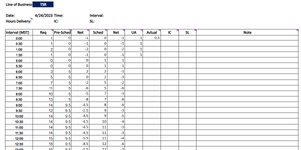
Data Set

This is how I want it to look like
1.

2.

4.
4.

 

[Peter_SSs]

Welcome to the MrExcel board!

1. I'm trying to return values from F1-L1 (Headers) to M2 as days of the week that has work schedule but i couldn't figure it out.

For that part, try this.

23 07 11.xlsm
	F	G	H	I	J	K	L	M
1	Sunday	Monday	Tuesday	Wednesday	Thursday	Friday	Saturday	Work Days
2	OFF						OFF	Mon, Tue, Wed, Thu, Fri
3	OFF						OFF	Mon, Tue, Wed, Thu, Fri
4				OFF	OFF			Sun, Mon, Tue, Fri, Sat
5					OFF	OFF		Sun, Mon, Tue, Wed, Sat
6					OFF	OFF		Sun, Mon, Tue, Wed, Sat
7	OFF	OFF						Tue, Wed, Thu, Fri, Sat
8					OFF	OFF		Sun, Mon, Tue, Wed, Sat
Headers

Cell Formulas
Range	Formula
M2:M8	M2	=TEXTJOIN(", ",,FILTER(LEFT(F$1:L$1,3),F2:L2<>"OFF"))

 

[keda duck]

For this question, I have another idea.

test.xlsx
	F	G	H	I	J	K	L	M
1	Sunday	Monday	Tuesday	Wednesday	Thursday	Friday	Saturday	Work Days
2	OFF						OFF	Mon, Tue, Wed, Thu, Fri
3	OFF						OFF	Mon, Tue, Wed, Thu, Fri
4				OFF	OFF			Sun, Mon, Tue, Fri, Sat
5					OFF	OFF		Sun, Mon, Tue, Wed, Sat
6					OFF	OFF		Sun, Mon, Tue, Wed, Sat
7	OFF	OFF						Tue, Wed, Thu, Fri, Sat
8					OFF	OFF		Sun, Mon, Tue, Wed, Sat
Sheet2

Cell Formulas
Range	Formula
M2:M8	M2	=TEXTJOIN(", ",,IF(F2:L2<>"OFF",LEFT(F$1:L$1,3),""))

 

[VhanLab]

Thank you so much! Both formulas worked for me. What if I want the value to return as the days they are off, which do I need to change in the formula for this to work?

 

[Peter_SSs]

Just change the "not equals" (<>) near the end of my formula to "equals" (=)

23 07 11.xlsm
	F	G	H	I	J	K	L	M
1	Sunday	Monday	Tuesday	Wednesday	Thursday	Friday	Saturday	Off Days
2	OFF						OFF	Sun, Sat
3	OFF						OFF	Sun, Sat
4				OFF	OFF			Wed, Thu
5					OFF	OFF		Thu, Fri
6					OFF	OFF		Thu, Fri
7	OFF	OFF						Sun, Mon
8					OFF	OFF		Thu, Fri
Headers (2)

Cell Formulas
Range	Formula
M2:M8	M2	=TEXTJOIN(", ",,FILTER(LEFT(F$1:L$1,3),F2:L2="OFF"))

 

[keda duck]

You can change the "not equals" (<>) near the end of my formula to "equals" (=)

test.xlsx
	F	G	H	I	J	K	L	M
1	Sunday	Monday	Tuesday	Wednesday	Thursday	Friday	Saturday	Work Days
2	OFF						OFF	Sun, Sat
3	OFF						OFF	Sun, Sat
4				OFF	OFF			Wed, Thu
5					OFF	OFF		Thu, Fri
6					OFF	OFF		Thu, Fri
7	OFF	OFF						Sun, Mon
8					OFF	OFF		Thu, Fri
Sheet2

Cell Formulas
Range	Formula
M2:M8	M2	=TEXTJOIN(", ",,IF(F2:L2="OFF",LEFT(F$1:L$1,3),""))