Search for date and penultimate date and numbers

Wojciech

New Member
Joined
May 13, 2018
Messages
26
Office Version
  1. 2021
Platform
  1. Windows
Hi,
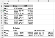
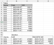
please help me write the formula. I am attaching a screenshot that shows the table and solution. The formula should be filled with the AAA or BBB (A13 and A14) and the formula should find the latest date (B13 and B14) and the number (number of kilometers) assigned to it (C13 and C14). The formula in D13,D14 finds the penultimate date and in E13 and E14 penultimate date number assigned to the dates.
 

Attachments

  • km.png
    km.png
    42 KB · Views: 5
So why does the function still work correctly after adding the third parameter CCC and the third searched row number 20? Please check the screenshot.

Edit: I think I understand now. These are the two lines we are looking for and they are calculated in "memory".
 

Attachments

  • km2.png
    km2.png
    36 KB · Views: 1
Upvote 0

Excel Facts

Which came first: VisiCalc or Lotus 1-2-3?
Dan Bricklin and Bob Frankston debuted VisiCalc in 1979 as a Visible Calculator. Lotus 1-2-3 debuted in the early 1980's, from Mitch Kapor.
When there is one AAA row in the table or I ask for a CCC parameter that does not exist in the table, the function throws errors. Please help me improve the function.

km.xlsx
ABCDEFG
1Table:
2NameDateKM
3AAA2023-09-0730019
4BBB2023-07-2724972
5BBB2023-08-0425695
6BBB2023-07-0723392
7
8
9 =INDEX(SORT(FILTER($B$2:$C$8,$A$2:$A$8=A13),1,-1),{1,1,2,2},{1,2,1,2})
10
11When there is one AAA row in the table or I ask for a CCC parameter that does not exist in the table, the function throws errors.
12Solution:
13inquiry:LastSecond to last
14AAA2023-09-0730019#ADR!#ADR!
15BBB2023-08-04256952023-07-2724972
16CCC#OBL!#OBL!#OBL!#OBL!
17
18The expected result.
19Solution:
20inquiry:LastSecond to last
21AAA2023-09-0730019
22BBB2023-08-04256952023-07-2724972
23CCC
24
km
Cell Formulas
RangeFormula
B21:E22,B14:E16B14=INDEX(SORT(FILTER($B$2:$C$6,$A$2:$A$6=A14),1,-1),{1,1,2,2},{1,2,1,2})
Dynamic array formulas.
 
Last edited:
Upvote 0
How about
Excel Formula:
=IFERROR(INDEX(SORT(FILTER($B$2:$C$6,$A$2:$A$6=A21),1,-1),{1,1,2,2},{1,2,1,2}),"")
 
Upvote 0

Forum statistics

Threads
1,215,267
Messages
6,123,964
Members
449,137
Latest member
yeti1016

We've detected that you are using an adblocker.

We have a great community of people providing Excel help here, but the hosting costs are enormous. You can help keep this site running by allowing ads on MrExcel.com.
Allow Ads at MrExcel

Which adblocker are you using?

Disable AdBlock

Follow these easy steps to disable AdBlock

1)Click on the icon in the browser’s toolbar.
2)Click on the icon in the browser’s toolbar.
2)Click on the "Pause on this site" option.
Go back

Disable AdBlock Plus

Follow these easy steps to disable AdBlock Plus

1)Click on the icon in the browser’s toolbar.
2)Click on the toggle to disable it for "mrexcel.com".
Go back

Disable uBlock Origin

Follow these easy steps to disable uBlock Origin

1)Click on the icon in the browser’s toolbar.
2)Click on the "Power" button.
3)Click on the "Refresh" button.
Go back

Disable uBlock

Follow these easy steps to disable uBlock

1)Click on the icon in the browser’s toolbar.
2)Click on the "Power" button.
3)Click on the "Refresh" button.
Go back
Back
Top