Search multiple exact strings in multiple columns

[Sebastian P]

Hello everyone,

I am new to this forum so pardon me if broke any rules through this post.

As the subject of the post states, I am trying to search multiple exact strings in multiple columns. Meaning in the attached file I am searching for certain strings (group names) in a range of cells (multiple columns)

The groups are as per below details:

PUBLIC
GTIS CMUK Windows Approval
GTIS CMUK Windows
UNIX-SUPPORT-FR
MIT Windows
MIT Unix
MIT Windows Approval
MIT Unix Approval
GTIS Hosting Platform Windows

PRIVATE
GTIS Hosting Platform Taurus Approval
GTIS Hosting Platform Taurus
GTIS Hosting Platform Atlas
GTIS Hosting Platform Atlas Approval

The formula I used is:
=IF(OR(ISNUMBER(SEARCH({"GTIS CMUK Windows Approval","GTIS CMUK Windows","UNIX-SUPPORT-FR","MIT Windows","MIT Unix","MIT Windows Approval","MIT Unix Approval","GTIS Hosting Platform Windows"},Table2[@[Group 1]:[Group 6]]))),"PUBLIC",IF(OR(ISNUMBER(SEARCH({"GTIS Hosting Platform Taurus Approval","GTIS Hosting Platform Taurus","GTIS Hosting Platform Atlas","GTIS Hosting Platform Atlas Approval"},Table2[@[Group 1]:[Group 6]]))),"PRIVATE","NONE"))

I have the following points for which I would need support:
1. Is the formula looking in the entire array A2 to A17, by using Table2[@[Group 1]:[Group 6]] in the syntax? I am asking this because:
------>The value returned in cells G4-G8 should be PUBLIC, but the formula does not find a match, though the UNIX-SUPPORT-FR group is in the PUBLIC category

2. How can adapt the formula to search for an exact match. From what I managed to figure out, because the formula does not look for an exact match, the following happens

------>The value in G9-G17 should be PRIVATE, but because the formula does not searches for an exact match, it returns PUBLIC
------>This happens because in one of the Group1 to Group 6 column there is a partial match of the searched text (bolded in below
------>"GTIS Hosting Platform Windows" -->this is PRIVATE
------>"GTIS Hosting Platform Atlas Approval"-->this should be PUBLIC

Thank you in advance,

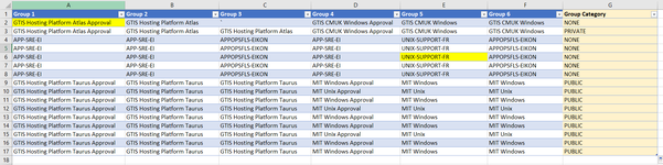
Column A Column B Column C Column D Column E Column F Column G
Group 1 Group 2 Group 3 Group 4 Group 5 Group 6 Group Category
GTIS Hosting Platform Atlas Approval GTIS Hosting Platform Atlas ` GTIS CMUK Windows Approval GTIS CMUK Windows GTIS CMUK Windows NONE
GTIS Hosting Platform Atlas Approval GTIS Hosting Platform Atlas GTIS Hosting Platform Atlas GTIS CMUK Windows Approval GTIS CMUK Windows GTIS CMUK Windows PRIVATE
APP-SRE-EI APP-SRE-EI APPOPSFLS-EIKON APP-SRE-EI UNIX-SUPPORT-FR APPOPSFLS-EIKON NONE
APP-SRE-EI APP-SRE-EI APPOPSFLS-EIKON APP-SRE-EI UNIX-SUPPORT-FR APPOPSFLS-EIKON NONE
APP-SRE-EI APP-SRE-EI APPOPSFLS-EIKON APP-SRE-EI UNIX-SUPPORT-FR APPOPSFLS-EIKON NONE
APP-SRE-EI APP-SRE-EI APPOPSFLS-EIKON APP-SRE-EI UNIX-SUPPORT-FR APPOPSFLS-EIKON NONE
APP-SRE-EI APP-SRE-EI APPOPSFLS-EIKON APP-SRE-EI UNIX-SUPPORT-FR APPOPSFLS-EIKON NONE
GTIS Hosting Platform Taurus Approval GTIS Hosting Platform Taurus GTIS Hosting Platform Taurus MIT Windows Approval MIT Windows MIT Windows PUBLIC
GTIS Hosting Platform Taurus Approval GTIS Hosting Platform Taurus GTIS Hosting Platform Taurus MIT Unix Approval MIT Unix MIT Unix PUBLIC
GTIS Hosting Platform Taurus Approval GTIS Hosting Platform Taurus GTIS Hosting Platform Taurus MIT Windows Approval MIT Windows MIT Windows PUBLIC
GTIS Hosting Platform Taurus Approval GTIS Hosting Platform Taurus GTIS Hosting Platform Taurus MIT Unix Approval MIT Unix MIT Unix PUBLIC
GTIS Hosting Platform Taurus Approval GTIS Hosting Platform Taurus GTIS Hosting Platform Taurus MIT Windows Approval MIT Windows MIT Windows PUBLIC
GTIS Hosting Platform Taurus Approval GTIS Hosting Platform Taurus GTIS Hosting Platform Taurus MIT Windows Approval MIT Windows MIT Windows PUBLIC
GTIS Hosting Platform Taurus Approval GTIS Hosting Platform Taurus GTIS Hosting Platform Taurus MIT Unix Approval MIT Unix MIT Unix PUBLIC
GTIS Hosting Platform Taurus Approval GTIS Hosting Platform Taurus GTIS Hosting Platform Taurus MIT Windows Approval MIT Windows MIT Windows PUBLIC
GTIS Hosting Platform Taurus Approval GTIS Hosting Platform Taurus GTIS Hosting Platform Taurus MIT Windows Approval MIT Windows MIT Windows PUBLIC

 

[StephenCrump]

Welcome to the Forum!

A simpler example, to illustrate why your formula is failing. Here, we're comparing four columns to six, hence two #N/A columns in the results. Occasionally you get lucky when the values line up - e.g. when "r", the third term of your search, is in column 3.

	A	B	C	D	E	F	G	H	I	J	K	L	M
1
2	Blah	Blah	Blah	Blah	Blah	Blah		#VALUE!	#VALUE!	#VALUE!	#VALUE!	#N/A	#N/A
3	Blah	Blah	r	Blah	Blah	Blah		#VALUE!	#VALUE!	1	#VALUE!	#N/A	#N/A
4	Blah	Blah	Blah	r	Blah	Blah		#VALUE!	#VALUE!	#VALUE!	#VALUE!	#N/A	#N/A
Sheet1

Cell Formulas
Range	Formula
H2:M4	H2	=SEARCH({"p","q","r","s"},A2:F2)
Dynamic array formulas.

Here's another way you could do this:

	A	B	C	D	E	F	G	H	I	J
1	Group 1	Group 2	Group 3	Group 4	Group 5	Group 6	Status		Public	Private
2	MIT Windows approval	Blah	Blah	Blah	Blah	Blah	Public		GTIS CMUK Windows Approval	GTIS Hosting Platform Taurus Approval
3	Blah	GTIS Hosting Platform Taurus	MIT Windows	Blah	Blah	Blah	Public		GTIS CMUK Windows	GTIS Hosting Platform Taurus
4	Blah	Blah	GTIS Hosting Platform Taurus	Blah	Blah	Blah	Private		UNIX-SUPPORT-FR	GTIS Hosting Platform Atlas
5	Blah	Blah	Blah	Blah	Blah	Blah	None		MIT Windows	GTIS Hosting Platform Atlas Approval
6									MIT Unix
7									MIT Windows Approval
8									MIT Unix Approval
9									GTIS Hosting Platform Windows
10
Sheet1

Cell Formulas
Range	Formula
G2:G5	G2	=IF(OR(COUNTIF(Table2[@[Group 1]:[Group 6]],Public)),"Public",IF(OR(COUNTIF(Table2[@[Group 1]:[Group 6]],Private)),"Private","None"))

Named Ranges
Name	Refers To	Cells
Private	=Sheet1!$J$2:$J$5	G2:G5
Public	=Sheet1!$I$2:$I$9	G2:G5

 

[Sebastian P]

Hi Stephen,

Thx so much for the answer. I have used Tables instead of Named Ranges, but indeed, much cleaner/readable/understandable formula.

I am still facing an issue, for which I have found a workaround, but not sure is the best solution.

I have used the following two formulas:

Group Category 1 --> formula used: =IF(OR(COUNTIF(Table2[@[Group 1]:[Group 6]],PUBLIC)),"PUBLIC",IF(OR(COUNTIF(Table2[@[Group 1]:[Group 6]],PRIVATE)),"PRIVATE","NONE"))

Group Category 2 --> formula used: =IF(OR(COUNTIF(Table2[@[Group 1]:[Group 3]],PUBLIC)),"PUBLIC",IF(OR(COUNTIF(Table2[@[Group 1]:[Group 3]],PRIVATE)),"PRIVATE",IF(OR(COUNTIF(Table2[@[Group 4]:[Group 6]],PUBLIC)),"PUBLIC",IF(OR(COUNTIF(Table2[@[Group 4]:[Group 6]],PRIVATE)),"PRIVATE","NONE"))))

and it returns as per below table:

Group 1	Group 2	Group 3	Group 4	Group 5	Group 6	Group Category 1	Group Category 2
GTIS Hosting Platform Atlas Approval	GTIS Hosting Platform Atlas	GTIS Hosting Platform Atlas	GTIS CMUK Windows Approval	GTIS CMUK Windows	GTIS CMUK Windows	PUBLIC	PRIVATE
GTIS Hosting Platform Atlas Approval	GTIS Hosting Platform Atlas	GTIS Hosting Platform Atlas	GTIS CMUK Windows Approval	GTIS CMUK Windows	GTIS CMUK Windows	PUBLIC	PRIVATE
APP-SRE-EI	APP-SRE-EI	APPOPSFLS-EIKON	APP-SRE-EI	UNIX-SUPPORT-FR	APPOPSFLS-EIKON	PUBLIC	PUBLIC
APP-SRE-EI	APP-SRE-EI	APPOPSFLS-EIKON	APP-SRE-EI	UNIX-SUPPORT-FR	APPOPSFLS-EIKON	PUBLIC	PUBLIC
GTIS Hosting Platform Taurus Approval	GTIS Hosting Platform Taurus	GTIS Hosting Platform Taurus	MIT Windows Approval	MIT Windows	MIT Windows	PUBLIC	PRIVATE
GTIS Hosting Platform Taurus Approval	GTIS Hosting Platform Taurus	GTIS Hosting Platform Taurus	MIT Unix Approval	MIT Unix	MIT Unix	PUBLIC	PRIVATE

My understanding as to why on rows 2, 3, 6, 7 there are different results between columns Group Category 1 and Group Category 2, is because the Group Category 1 formula takes one random value from any of the Group 1 to Group 6 values.
Group Category 2 formula, though probably also takes any random value, because there is a split of IFs (first looks in Group1 to Group3, and after it looks in Group4 to Group6) , it will return PRIVATE.

I am trying to understand if there is any way in which the formula can search in order from Group 1 to Group 6 and return PRIVATE or PUBLIC, based on first value found

Below are the Tables I used. First one named PRIVATE and the second one named PUBLIC

PRIVATE

GTIS Hosting Platform Taurus Approval

GTIS Hosting Platform Taurus

GTIS Hosting Platform Atlas

GTIS Hosting Platform Atlas Approval

PUBLIC

GTIS CMUK Windows Approval

GTIS CMUK Windows

UNIX-SUPPORT-FR

MIT Windows

MIT Unix

MIT Windows Approval

MIT Unix Approval

GTIS Hosting Platform Windows

 

[StephenCrump]

I think this is what you mean?

	A	B	C	D	E	F	G	H	I	J	K
1	Group 1	Group 2	Group 3	Group 4	Group 5	Group 6	Status	Column1		Public	Private
2	MIT Windows approval	Blah	Blah	Blah	Blah	Blah	Public	Public		GTIS CMUK Windows Approval	GTIS Hosting Platform Taurus Approval
3	Blah	GTIS Hosting Platform Taurus	MIT Windows	Blah	Blah	Blah	Public	Private		GTIS CMUK Windows	GTIS Hosting Platform Taurus
4	Blah	Blah	GTIS Hosting Platform Taurus	Blah	Blah	Blah	Private	Private		UNIX-SUPPORT-FR	GTIS Hosting Platform Atlas
5	Blah	Blah	Blah	Blah	Blah	Blah	None	None		MIT Windows	GTIS Hosting Platform Atlas Approval
6										MIT Unix
7										MIT Windows Approval
8										MIT Unix Approval
9										GTIS Hosting Platform Windows
10
11										Combined
12										GTIS CMUK Windows Approval	Public
13										GTIS CMUK Windows	Public
14										UNIX-SUPPORT-FR	Public
15										MIT Windows	Public
16										MIT Unix	Public
17										MIT Windows Approval	Public
18										MIT Unix Approval	Public
19										GTIS Hosting Platform Windows	Public
20										GTIS Hosting Platform Taurus Approval	Private
21										GTIS Hosting Platform Taurus	Private
22										GTIS Hosting Platform Atlas	Private
23										GTIS Hosting Platform Atlas Approval	Private
Sheet1

Cell Formulas
Range	Formula
G2:G5	G2	=IF(OR(COUNTIF(Table2[@[Group 1]:[Group 6]],Public)),"Public",IF(OR(COUNTIF(Table2[@[Group 1]:[Group 6]],Private)),"Private","None"))
H2:H5	H2	=LET(p,VLOOKUP(Table2[@[Group 1]:[Group 6]],Combined,2,),TAKE(FILTER(p,ISTEXT(p),"None"),,1))

Named Ranges
Name	Refers To	Cells
Combined	=Sheet1!$J$12:$K$23	H2:H5
Private	=Sheet1!$K$2:$K$5	G2:G5
Public	=Sheet1!$J$2:$J$9	G2:G5

 

[StephenCrump]

Or with just the one lookup table:

	A	B	C	D	E	F	G	H	I	J	K
1	Group 1	Group 2	Group 3	Group 4	Group 5	Group 6	Status 1	Status 2		Combined
2	MIT Windows approval	Blah	Blah	Blah	Blah	Blah	Public	Public		GTIS CMUK Windows Approval	Public
3	Blah	GTIS Hosting Platform Taurus	MIT Windows	Blah	Blah	Blah	Public	Private		GTIS CMUK Windows	Public
4	Blah	Blah	GTIS Hosting Platform Taurus	Blah	Blah	Blah	Private	Private		UNIX-SUPPORT-FR	Public
5	Blah	Blah	Blah	Blah	Blah	Blah	None	None		MIT Windows	Public
6										MIT Unix	Public
7										MIT Windows Approval	Public
8										MIT Unix Approval	Public
9										GTIS Hosting Platform Windows	Public
10										GTIS Hosting Platform Taurus Approval	Private
11										GTIS Hosting Platform Taurus	Private
12										GTIS Hosting Platform Atlas	Private
13										GTIS Hosting Platform Atlas Approval	Private
Sheet1

Cell Formulas
Range	Formula
G2:G5	G2	=LET(p,IFERROR(VLOOKUP(Table2[@[Group 1]:[Group 6]],Combined,2,),""),IF(OR(p="Public"),"Public",IF(OR(p="Private"),"Private","None")))
H2:H5	H2	=LET(p,VLOOKUP(Table2[@[Group 1]:[Group 6]],Combined,2,),TAKE(FILTER(p,ISTEXT(p),"None"),,1))

Named Ranges
Name	Refers To	Cells
Combined	=Sheet1!$J$2:$K$13	G2:H5

 

[Sebastian P]

HI Stephen,

Thx once again. The H2 formula does what I needed.

Do you mind walking me through the formula a little bit, so I understand how it works?

 

[StephenCrump]

Do you mind walking me through the formula a little bit, so I understand how it works?

Just break it down into steps:

	A	B	C	D	E	F	G	H	I	J	K
1	Group 1	Group 2	Group 3	Group 4	Group 5	Group 6	Status 1	Status 2		Combined
2	MIT Windows approval	Blah	Blah	Blah	Blah	Blah	Public	Public		GTIS CMUK Windows Approval	Public
3	Blah	GTIS Hosting Platform Taurus	MIT Windows	Blah	Blah	Blah	Public	Private		GTIS CMUK Windows	Public
4	Blah	Blah	GTIS Hosting Platform Taurus	Blah	Blah	Blah	Private	Private		UNIX-SUPPORT-FR	Public
5	Blah	Blah	Blah	Blah	Blah	Blah	None	None		MIT Windows	Public
6										MIT Unix	Public
7										MIT Windows Approval	Public
8	H3, in steps									MIT Unix Approval	Public
9	VLOOKUP									GTIS Hosting Platform Windows	Public
10	#N/A	Private	Public	#N/A	#N/A	#N/A				GTIS Hosting Platform Taurus Approval	Private
11										GTIS Hosting Platform Taurus	Private
12	Filter									GTIS Hosting Platform Atlas	Private
13	Private	Public								GTIS Hosting Platform Atlas Approval	Private
14
15	Take first
16	Private
17
Sheet1

Cell Formulas
Range	Formula
G2:G5	G2	=LET(p,IFERROR(VLOOKUP(Table2[@[Group 1]:[Group 6]],Combined,2,),""),IF(OR(p="Public"),"Public",IF(OR(p="Private"),"Private","None")))
H2:H5	H2	=LET(p,VLOOKUP(Table2[@[Group 1]:[Group 6]],Combined,2,),TAKE(FILTER(p,ISTEXT(p),"None"),,1))
A10:F10	A10	=VLOOKUP(A3:F3,Combined,2,)
A13:B13	A13	=FILTER(A10#,ISTEXT(A10#),"None")
A16	A16	=TAKE(A13#,,1)
Dynamic array formulas.

Named Ranges
Name	Refers To	Cells
Combined	=Sheet1!$J$2:$K$13	A10, G2:H5

 

[Sebastian P]

Thx Stephen.

One more question please.

If on one row there are groups belonging to both Private and Public:
-return each different value(Private and Public) in a different column
-the order of the returned values to be descending based on the number of iterations(if there are 3 Private groups and 2 Public groups, return in Private in column G and Public in column H)
-----> in below example, Groups 1, 2, 3 are PRIVATE (so 3 iterations) and Groups 4, 5 are PUBLIC --> so PRIVATE in column G and PUBLIC in column H

Group 1	Group 2	Group 3	Group 4	Group 5	Group 6	Group Category 1 column G	Group Category 2 column H
GTIS Hosting Platform Atlas Approval	GTIS Hosting Platform Atlas	GTIS Hosting Platform Atlas	GTIS CMUK Windows Approval	APP-SRE-EI	GTIS CMUK Windows	PRIVATE	PUBLIC

 

[StephenCrump]

Perhaps like this?

I have assumed that if there are equal numbers of Public/Private the results should show Public and Private in that order.

	A	B	C	D	E	F	G	H	I	J	K
1	Group 1	Group 2	Group 3	Group 4	Group 5	Group 6	Status 1	Status 2		Combined
2	MIT Windows approval	Blah	Blah	Blah	Blah	Blah	Public			GTIS CMUK Windows Approval	Public
3	Blah	GTIS Hosting Platform Taurus	MIT Windows	Blah	Blah	Blah	Public	Private		GTIS CMUK Windows	Public
4	Blah	Blah	GTIS Hosting Platform Taurus	Blah	Blah	Blah	Private			UNIX-SUPPORT-FR	Public
5	Blah	Blah	Blah	Blah	Blah	Blah				MIT Windows	Public
6	Blah	Blah	MIT Windows	Blah	Blah	Blah	Public			MIT Unix	Public
7	GTIS Hosting Platform Taurus	GTIS Hosting Platform Taurus			MIT Unix	MIT Unix	Public	Private		MIT Windows Approval	Public
8										MIT Unix Approval	Public
9										GTIS Hosting Platform Windows	Public
10										GTIS Hosting Platform Taurus Approval	Private
11										GTIS Hosting Platform Taurus	Private
12										GTIS Hosting Platform Atlas	Private
13										GTIS Hosting Platform Atlas Approval	Private
14
Sheet1

Cell Formulas
Range	Formula
G2:G7	G2	=LET(p,{"Public";"Private"},n,BYROW(IFERROR(VLOOKUP(Table2[@[Group 1]:[Group 6]],Combined,2,),"None")=p,LAMBDA(r,SUM(--r))),IF(MAX(n)=0,"",INDEX(SORTBY(p,n,-1),1)))
H2:H7	H2	=LET(p,{"Public";"Private"},n,BYROW(IFERROR(VLOOKUP(Table2[@[Group 1]:[Group 6]],Combined,2,),"None")=p,LAMBDA(r,SUM(--r))),IF(MIN(n)=0,"",INDEX(SORTBY(p,n,-1),2)))

Named Ranges
Name	Refers To	Cells
Combined	=Sheet2!$J$2:$K$13	G2:H7

 

[Sebastian P]

Hi Stephen,

Sorry for the delayed response.

Formula does almost what I need

So, from your formula, if I remove INDEX, it will return #SPILL!

G2:G7

G2

=LET(p,{"Public";"Private"},n,BYROW(IFERROR(VLOOKUP(Table2[@[Group 1]:[Group 6]],Combined,2,),"None")=p,LAMBDA(r,SUM(--r))),IF(MAX=0,"",INDEX(SORTBY(p,n,-1),1)))

If I am using A3:F3 instead of Table2[@[Group 1]:[Group 6]] I will get as per below

=LET(p,{"Public";"Private"},n,BYROW(IFERROR(VLOOKUP(A3:F3,COMBINED2,2),"None")=p,LAMBDA(r,SUM(--r))),IF(MAX=0,"",SORTBY(p,n,1)))

Private

Public

What I would want is to have the spilled values go into separate columns, something like below

=TRANSPOSE(LET(p,{"Public";"Private"},n,BYROW(IFERROR(VLOOKUP(A3:F3,COMBINED2,2),"None")=p,LAMBDA(r,SUM(--r))),IF(MAX=0,"",SORTBY(p,n,1))))
Private	Public

The issue is that, even with TRANSPOSE, if I am using Table2[@[Group 1]:[Group 6]] instead of A3:F3, it will still return #SPILL!