Searching for data on another sheet

[thevaper]

Hello

I need help in creating a log for our business. Basically, we have different pricing for our physical store and online store. I'm trying to get a formula to work on a cell that will look for the price of the online/physical store when I input a code. Please see the details below.

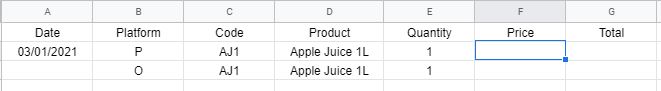
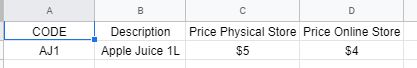
The first screenshot is on Sheet 1 which is the main page where we log the sale. What we want to do is on F2. We're looking for a formula that would use the code on B2 (P=Physical store - column c on sheet 2, O=online store - column D on sheet 2), to look for the price of the product code on sheet 1 C2. For example 2nd row should pull the price of $5 (from sheet 2 c3) when B2 is P and the product code on C2 is entered.

Thank you for your answer

 

[Michael M]

How about

=IF(B2="P", VLOOKUP(C2,Sheet2!A2:D2,3,0)*E2,VLOOKUP(C2,Sheet2!A2:D2,4,0)*E2)

 

[jtakw]

Hi,

Here's one way.

You didn't specify if the "Quantity" is a factor, so I included both, Change Sheet810 to Sheet2:

Book3.xlsx
	A	B	C	D	E	F	G
1		Platform	Code		Quantity	Price	w/ Quantity
2		P	AJ1		1	5	5
3		O	AJ1		1	4	4
4		P	OJ1		5	5.5	27.5
5		O	OJ1		9	4.5	40.5
6
Sheet807

Cell Formulas
Range	Formula
F2:F6	F2	=IFERROR(INDEX(IF(B2="P",Sheet810!C$1:C$10,Sheet810!D$1:D$10),MATCH(C2,Sheet810!A$1:A$10,0)),"")
G2:G6	G2	=IFERROR(INDEX(IF(B2="P",Sheet810!C$1:C$10,Sheet810!D$1:D$10),MATCH(C2,Sheet810!A$1:A$10,0))*E2,"")

Book3.xlsx
	A	B	C	D
1	Code		Price Physical	Price Online
2	AJ1		$5	$4
3	OJ1		$5.50	$4.50
Sheet810

 

[jtakw]

Adding another way for VLOOKUP, again change Sheet810 to Sheet2:

Book3.xlsx
	A	B	C	D	E	F	G
1		Platform	Code		Quantity	Price	w/ Quantity
2		P	AJ1		1	5	5
3		O	AJ1		1	4	4
4		P	OJ1		5	5.5	27.5
5		O	OJ1		9	4.5	40.5
6
Sheet807

Cell Formulas
Range	Formula
F2:F5	F2	=IFERROR(VLOOKUP(C2,Sheet810!A$2:D$10,IF(B2="P",3,4),0),"")
G2:G6	G2	=IFERROR(VLOOKUP(C2,Sheet810!A$2:D$10,IF(B2="P",3,4),0)*E2,"")

Book3.xlsx
	A	B	C	D
1	Code		Price Physical	Price Online
2	AJ1		$5	$4
3	OJ1		$5.50	$4.50
Sheet810

 

[thevaper]

@Michael M and @jtakw Thank you so much for the answer. The formula worked pretty well. We just made some adjustments to match the range on our file. You guys are great!

 

[Michael M]

Glad WE could help.. .as a matter of interest, which formula did you go with ??

 

[jtakw]

You're welcome, thanks for feedback, glad we can help.