Selective Transpose

[isasa74]

Hi Guys,

I need help please.
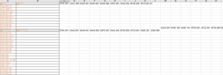
I have a long list of values for that I need to transpose, however I need a formula that can dynamically select the number of lines to transpose.

Mine it's a list of part numbers, with the Parent part numbers starting by 1 and Childs part numbers randomly starting by any other number (4-5-6 etc.)
In the list for each Parent there is a variable number of Childs parts.

The Formula should look at the Parent and transposing all the Childs in the same row of the Parent.
I'm ok as excel user but I'm not up to this level, any help is welcome and a bit of code will do as well , however a solution by a formula is preferred.


Thanks in advance

1Blueparent	after the Formula -->	1Blueparent	4child1	6child2
4child1
6child2
1Redparent		1Redparent	5child1	etc.
5child1

 

[Special-K99]

I see 3 patterns so you need to decide which of these is correct (if any) or define what constitutes the change of parent

The list starts with a parent and continues with a list of children until one of these things happens to indicate a new parent

1. All parents have numbers that begin with a 1
2. The word parent appears in the next row or
3. The first number encountered in the row below is less than the first number encountered in the current row, e.g. reading down 1, 4, 6, 1 (new parent).

Or is it something else that defines a change of parent?

 

[Special-K99]

This works

Data in column A
Result in column B going horizontally across the sheet
This assumes a new parent is indicated by the first digit in a row being 1
If this is not the case then you need to change this line

        If Val(Left(Cells(i, 1), 1)) =1 Then

to define what constitutes a new parent

Sub k1()
lastrow = Worksheets("Sheet1").Cells(Rows.Count, "A").End(xlUp).Row
i = 0
k = 999
l = 1
While i <> lastrow
i = i + 1
        If Val(Left(Cells(i, 1), 1)) =1 Then
        j = i
        l = 2
        k = Val(Left(Cells(i, 1), 1))
    Else
        l = l + 1
    End If
    Cells(j, l) = Cells(i, 1)
        k = Val(Left(Cells(i, 1), 1))
Wend
End Sub

 

[isasa74]

This works

Data in column A
Result in column B going horizontally across the sheet
This assumes a new parent is indicated by the first digit in a row being 1
If this is not the case then you need to change this line

        If Val(Left(Cells(i, 1), 1)) =1 Then

to define what constitutes a new parent

Sub k1()
lastrow = Worksheets("Sheet1").Cells(Rows.Count, "A").End(xlUp).Row
i = 0
k = 999
l = 1
While i <> lastrow
i = i + 1
        If Val(Left(Cells(i, 1), 1)) =1 Then
        j = i
        l = 2
        k = Val(Left(Cells(i, 1), 1))
    Else
        l = l + 1
    End If
    Cells(j, l) = Cells(i, 1)
        k = Val(Left(Cells(i, 1), 1))
Wend
End Sub

Hi Special-K99

thanks a lot for helping me .

to reply your questions first:

1. All parents have numbers that begin with a 1 --> Correct!, all Parent Starts with 1* and doesn't not end with an "S" and/or with "S.*" where the STAR is a number (e.g. S.2. S.3, etc.) apologize this requirement just popped up now.

2. The word parent appears in the next row or--> Word Parent won't appear at all, parent part numbers consist in an alphanumerical code whose logic is irrelevant to the exercise, I used the word parent just to avoid the real part number

3. The first number encountered in the row below is less than the first number encountered in the current row, e.g. reading down 1, 4, 6, 1 (new parent). --> not sure I understand the question

Concerning the code

I ran the code which according to the debug errored in the line Cells(j, l) = Cells(i, 1)

thanks again so much

 

[Peter_SSs]

I suggest that you update your Account details (or click your user name at the top right of the forum) so helpers always know what Excel version(s) & platform(s) you are using as the best solution often varies by version. (Don’t forget to scroll down & ‘Save’)

 

[Special-K99]

Answer to question 3 is answered in question 1 - all parents have a 1 at the beginning
for question 3, as soon as a 1 is encountered in the next row it indicates the start of a parent

Code worked ok for me.

Do this.
Start with a blank sheet
Put the values EXACTLY as you've given them in your example (but only the first column, not the results you want) - put those values in column A of the blank sheet.
Alt-11 - Paste the code
Run the code

On Sheet1 rows 1 and 4 have entries in columns B C D as per your requested

 

[isasa74]

It works for me too, thanks!

the only uncovered thing it's the additional criteria :

all Parent Starts with 1* and doesn't end with an "S" and/or with "S.*" where the STAR is a number (e.g. S.2. S.3, etc.) apologize this requirement just popped up now.

is it anything that can be fixed easily please?

 

[Special-K99]

Are you saying you have data that
starts with a 1but MAY not be a parent (because of the ending S or S.*) ?

 

[isasa74]

yes precisely, to be parent other that starting with 1* another condition is not ending in S or S* where the star after the S is a number.

I also have noticed 2 issues which will be clearer by looking at the screenshot

1) The Parent is copied in the next column too as it was a Child, consequentially I have it repeated twice, the original and a copy in the next column .
2) In case of long list of Childs (apparently when more than 10), Childs after the first 10 are copied one row above of the other Childs.

 

[Peter_SSs]

I need a formula ...

You originally asked for a formula to do this, but did not take up my suggestion for you to included your Excel version(s) in your account details so we still do not know what that is.
As an example, if you have Excel 365, something like this, copied down might get you close to what you want?

isasa74.xlsm
	A	B	C	D	E
1	1Blueparent	1Blueparent	4child1	6child2
2	4child1
3	6child2
4	1Redparent	1Redparent	5child1
5	5child1
6
Sheet1

Cell Formulas
Range	Formula
B1:D1,B4:C4,B2:B3,B5	B1	=IF(LEFT(A1,1)="1",TRANSPOSE(A1:INDEX(A1:A$100,IFNA(MATCH("1*",A2:A$100,0),COUNTA(A1:A$100)))),"")
Dynamic array formulas.

As well as updating your account details, if providing more sample data, please investigate XL2BB for providing sample data to make it easier for helpers by not having to manually type out sample data to test with.