Simple Index function drag down to change the row value accordingly

[ahme0740]

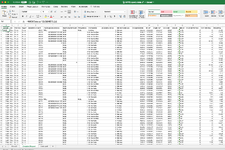
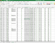
Hi, I have a pretty simple function. Context: I have 1 excel file and I'm trying to compile data onto one of the sheets (detailed report) from another sheet (data pull). I have some additional columns with formulas in the detailed report sheet that I don't want to overnight by copy pasting the data from the data pull sheet. The data pull sheet will be different every time (can't use VLOOKUP because there isn't something that would remain the same). I'm querying the data from a pharmacy database and depending on the time and parameters I use the query, the stores, order numbers, prescription numbers, etc would always be different. But I need to column names on detailed report sheet to stay as what I set them to but I want to pull the data for the relevant columns from the data I paste into the data pull sheet. I have data in columns A to R in the data pull sheet and A to T in the detailed report sheet (the two additional columns fall in the middle of the sheet). Anyways so I decided to use an INDEX function (hope this is correct), I'm okay with doing one function per column and dragging it down to reduce the complexity of the formula. So for Column A (named StoreId in A1), so from A2 down to however many rows the SQL query pulls for the given data pull, this is the formula I have =INDEX('Data pull'!$1:$1048576,2,1)

When I drag it down I want it to say =INDEX('Data pull'!$1:$1048576,3,1) for cell A3, =INDEX('Data pull'!$1:$1048576,4,1) for cell A4 and so on. If possible I would also like it to not display anything (blank cell) if I drag it all the way down and there are no records in that row from the data pull sheet. Is this even possible? I'm sure it is, but I'm very confused *crying face*

Right now when I drag it down it just copies =INDEX('Data pull'!$1:$1048576,2,1) down all the way and doesn't change anything. Please help!!! Thank you in advance

 

[ahme0740]

Also, some of the cells have the value NULL written in them, when I enter the formula in those cells, it just shows me the formula in the cell instead of the word NULL. I need to see NULL where it should be NULL. There are other cells that are blank, I also need to see them as blank. The blank ones also just show the formula written as =INDEX('Data pull'!$1:$1048576,X,Y) (X and Y being the relevant rows and columns). Same thing happens with basically any cell that has non numerical values. Like one of them has a date in the following format: 2023-08-01 15:53:58.000 and when I enter the formula with the relevant row and column it still just shows the formula instead of the value.

I am pretty sure I'm doing something very wrong I just can't figure it out

 

[awoohaw]

would you be kind enough to use the xl2bb add in and post miniworksheets of your data (sanitize for security).
The way you've presented your question means the forum must try to recreate your scenario instead of just trying to find you a solution.
The xl2bb add link is below. If you cannot use that then please post as tables. An image (screenshot) is minimally helpful since the forum must still reenter all your data and could have typos. You only need 10-20 rows of data to usually give enough information to work out a solution.

Please help the forum help you.

Thanks in advance.

 

[ahme0740]

Sure, also I troubleshooted. It was a csv file so the formulas weren't working. But the NULL is now showing as NULL and the blank ones are showing as 0, I'd like blank to show as blank though. I will attach the file, it's all from our test server so no PHI in here

 

[ahme0740]

Ugh, can't actually attach the file right now, permissions on this laptop won't let me download it. Will do it tonight at home. I can attach a screenshot so you can see what I'm talking about now.

 

[ahme0740]

Please see screenshots

 

[ahme0740]

I will attach the mini sheet in a few hours!

 

[awoohaw]

I will attach the mini sheet in a few hours!

you can also just post as a table. Highlight the data cells, copy, come to Mr. Excel Forum and paste.

 

[ahme0740]

StoreId	City	Province	Region	StoreWorkOrderId	EmployeeDiscountCode	MaxPaymentAmount	PrePayMode	PrePayMode	DeliveryRouteType
5538	NULL	NULL	NULL	86307​	NULL	NULL	NULL	In Store	2​
5538​	NULL	NULL	NULL	86306​	6006438207358160​	NULL	0​	Online-Confirm	2​
5538​	NULL	NULL	NULL	86308​	6006438207358160​	NULL	0​	Online-Confirm	2​
5538​	NULL	NULL	NULL	86308​	6006438207358160​	NULL	0​	Online-Confirm	2​
5538​	NULL	NULL	NULL	86310​	6006438207358160​	NULL	0​	Online-Confirm	2​
5538​	NULL	NULL	NULL	86310​	6006438207358160​	NULL	0​	Online-Confirm	2​
5564​	NULL	NULL	NULL	86255​	0​	NULL	1​	Online-Auto	1​
5564​	NULL	NULL	NULL	86255​		NULL	1​	Online-Auto	1​
5540​	NULL	NULL	NULL	75700​		NULL	1​	Online-Auto	2​

 

[awoohaw]

There are more efficient ways than using the INDEX function as you have it. But here a suggestion for that:

Instead of hard coding the row number (you have 2 copied all the way down) in the formula you need to create a way to automatically increment the row number.
you can do this with the ROW("cellref") function which returns the current row the referenced cell is in (and you can reference it in the same cell
for instance:
in cell A2 use this formula.

=INDEX('Data pull'!$1:$1048576,row(A2),1)

But that is not a good idea, you are killing your processing by reading an entire column.
I would suggest doing a COUNTA function on column A in the data sheet only to a number of ROWS that you probably will never exceed (maybe 25000? - you know this better than me). and combine that with SEQUENCE (starting at 2).

=INDEX('Data pull'!A$1:A$25000,sequence(25000,1,2,1),1)

But, there are other options.
Power Query will allow you to just keep data worksheets in a "repository" that you just refresh the worksheet and it will read the new file for you.

The choosecols function is quick and easy
Suppose you want columns A-K, N,P,S,T

=CHOOSECOLS('Data pull'!$A$1:$T$25000,1,2,3,4,5,6,7,8,9,10,11,12,14,16,17)

This video explains new ways to manipulate arrays of data.