Skip a column help

[chef855]

Hi there!

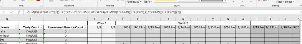
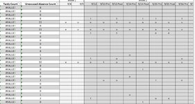
I've dug around Google and I cannot get this to work at all. I'm trying to track attendance for one class that's split. So students might attend before lunch, but not after lunch or vice versa. I have my columns set as such: H2 would say 9/14 Pre and then I2 would say 9/14 Post. I'm trying to get it so that it counts only one instance. So if a student was absent for both halves it's one absence in the total, not 2. Hope this makes sense. I've tried doing a few different formulas and ideas, but nothing that seems to do what I'm looking for.

 

[jasonb75]

Are you just looking at 2 columns, or are you looking at pairs of columns over a wider range?

If it is a wider range are they consecutive columns, or is there other information between them?

 

[chef855]

It's going to be an ongoing spreadsheet over the semester as we are tasked with tracking student tardies... PITA! It's pairs of columns over a longer range

 

[jasonb75]

Based on how you have described it, I would try something like this. I've only used 3 pairs of columns in the example but it can be expanded as needed.

Book1
	F	G	H	I	J	K	L	M
2	3		9/14 Pre	9/14 Post	9/15 Pre			9/16 Post
Sheet7

Cell Formulas
Range	Formula
F2	F2	=SUM(IF(FREQUENCY(IF($H2:$M2<>"",COLUMN($H2:$M2)),IF(MOD(COLUMN($H2:$M2),2),COLUMN($H2:$M2))),1))

 

[chef855]

Okay! I guess this is where I get stuck. Where would I increase the columns it counts? Or just wherever it says $M$2, put in my last column?

 

[jasonb75]

wherever it says $M$2, put in my last column?

Not as stuck as you thought, that's exactly how you would do it.

One other thing that I forgot to mention is that the formula is based on each pair starting in an even numbered column (H, J, L, N, etc) if the pairs are starting in an odd numbered column then you will need to use this one instead. Almost the same, but has an =0 check on the column pairs which is not used in the other one.

=SUM(IF(FREQUENCY(IF($I2:$N2<>"",COLUMN($I2:$N2)),IF(MOD(COLUMN($I2:$N2),2)=0,COLUMN($I2:$N2))),1))

 

[chef855]

Not as stuck as you thought, that's exactly how you would do it.

One other thing that I forgot to mention is that the formula is based on each pair starting in an even numbered column (H, J, L, N, etc) if the pairs are starting in an odd numbered column then you will need to use this one instead. Almost the same, but has an =0 check on the column pairs which is not used in the other one.

=SUM(IF(FREQUENCY(IF($I2:$N2<>"",COLUMN($I2:$N2)),IF(MOD(COLUMN($I2:$N2),2)=0,COLUMN($I2:$N2))),1))

I plugged it into my spreadsheet and now I'm getting a #value error.

 

[jasonb75]

I can't see any reason for that to happen. Do you have any #VALUE! errors anywhere in the columns H:AZZ ?

 

[chef855]

I can't see any reason for that to happen. Do you have any #VALUE! errors anywhere in the columns H:AZZ ?

I don't see any?

 

[jasonb75]

I've tried the exact formula that you have in your screen capture and don't get any errors.

Does it work correctly for you with a smaller range like the one in the example formula that I posted?