SMALL function returning 2 values

[brownrice]

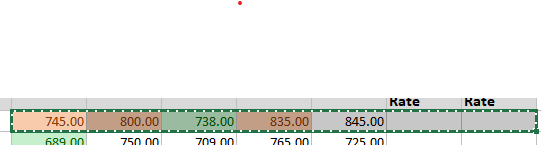
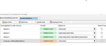
Hi folks, I am trying to use the SMALL function in a conditional statement to highlight only the 2nd smallest value in a row. In the same array I am using a contitional successfully to highlight the lowest value using "bottom 1."
When I add SMALL (=SMALL(e2:k2,2)) to return the 2nd smallest value, though, it returns both 2nd and 3rd smallest values. Not sure what I am doing wrong! Thanks!
Also do you know how to stop Excel from "helpfully" adding formula values when I move the arrow keys as I am writing a formula? It is just dumping random stuff in there! All I want to do is move the cursor. Thank you!

 

[RoryA]

Press f2 while editing.

Either you have two matching values, or you forgot to make the ranges absolute, I suspect.

 

[brownrice]

I don't have matching values, they are all different. Now it is returning everything except the highest value! I am not able to upload the mini-sheet because I can't find 'XL2BB" add in, but I included an image. the orange highlight is what is supposed to be only 2nd lowest value. The green, the lowest value, works fine.

 

[Joe4]

Did you make the range absolute, like Rory said?

If you are applying your original formula to all the columns in that row, you need to make the column part of your references absolute by changing this:

=SMALL(e2:k2,2)

to this:

=SMALL($e2:$k2,2)

See here for a detailed explanation of relative, absolute, and mixed range references.

Excel Formulas: Relative and Absolute Cell References

Learn the difference between a relative absolute cell reference in Excel and an absolute cell reference in Excel in this free lesson.

edu.gcfglobal.org

 

[brownrice]

Did you make the range absolute, like Rory said?

If you are applying your original formula to all the columns in that row, you need to make the column part of your references absolute by changing this:

=SMALL(e2:k2,2)

to this:

=SMALL($e2:$k2,2)

See here for a detailed explanation of relative, absolute, and mixed range references.

Excel Formulas: Relative and Absolute Cell References

Learn the difference between a relative absolute cell reference in Excel and an absolute cell reference in Excel in this free lesson.

edu.gcfglobal.org

Yes, that actually made it worse. Now it's highglighting the whole row. Not sure what I am doing wrong, is there maybe a different formula I can use? I have a lot of rows to apply this to. thanks for your help!

 

[Joe4]

Whoops, I think there needs to be another part of that formula, if we want to check if the value in that cell is the second smallest in that range.

If you select the range E2:K2, and then apply this Conditional Formatting formula:

=SMALL($E2:$K2,2)=E2

and then choose your formatting option, it should format the second smallest value in that range.

 

[brownrice]

Wouldn't that only check cell E2 though? I have a range of cells, I want to highlight the lowest rate, then also the 2nd lowest rate in that range. I assume I need 2 rules for that, and the 2nd lowest rule should be run after it checks for the lowest. Are the rules interfering with each other? I am just not sure why the original formula, which should give me only the 2nd lowest value, isn't working. I guess I could just change my original conditional to give me the bottom 2 rates instead, but that isn't quite what I'm looking for! I saw another solution that used an IF statement, but that seems to me like it shouldn't be necessary.

 

[MARK858]

Wouldn't that only check cell E2 though?

No, the E2 isn't absolute

Book1
	C	D	E	F	G	H	I	J	K
2	15		20	17	18	21	12	15	16
3	8		10	14	20	9	7	8	15
4	10		13	14	15	10	18	11	1
5	6		8	20	20	6	14	3	13
6	6		13	8	20	16	2	6	13
7	5		17	15	13	5	14	19	2
8	9		11	9	15	7	19	12	14
9	3		19	10	5	3	4	2	7
Sheet1

Cell Formulas
Range	Formula
C2:C9	C2	=SMALL(E2:K2,2)

Cells with Conditional Formatting
Cell	Condition		Cell Format	Stop If True
E2:K9	Expression	=SMALL($E2:$K2,2)=E2	text	NO

 

[Joe4]

Wouldn't that only check cell E2 though?

By NOT using the dollar sign in front of that column reference, it allows that one to float.

So, if you first select the range E2:K2, and then apply the formula I gave you hear is what Excel will actually do:

On cell E2: =SMALL($E2:$K2,2)=E2
On cell G2: =SMALL($E2:$K2,2)=G2
On cell H2: =SMALL($E2:$K2,2)=H2
etc.

See the pattern?

If you read the link I gave you, it will explain how it works but locking/not-locking certain column references.

 

[MARK858]

On cell E2: =SMALL($E2:$K2,2)=E2
On cell G2: =SMALL($E2:$K2,2)=F2
On cell H2: =SMALL($E2:$K2,2)=G2
etc.

Hi Joe, are you sure those references are correct?