Split row into two rows, one header and one line row

rrmando18

New Member
Joined
Sep 13, 2022
Messages
8
Office Version
  1. 365
Platform
  1. Windows
Good afternoon party people...hope everyone is doing great. I have been searching the forums but have not found anything yet. We are going to have between 100-200 rows at a time, one invoice per row, that we need to split into two separate rows so we can import into our ERP. We need to create one header row and one line row for each invoice row.

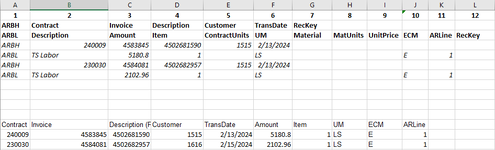
Below is an example. The top part is what we're trying to get to. That is the import template we need to use. ARBH is the header row. ARBL is the line row. On the bottom portion, Contract, Invoice, Description, Customer, TransDate need to go on the header row (ARBH row). Amount, Item, UM, ECM and ARLine need to go on the line row (ARBL row).

Any suggestions? Thank you for your help.

1711408252851.png
 

Attachments

  • 1711407929033.png
    1711407929033.png
    22.1 KB · Views: 2

Excel Facts

Can a formula spear through sheets?
Use =SUM(January:December!E7) to sum E7 on all of the sheets from January through December
you could try this code:
VBA Code:
Sub rrmando18()
Dim srcsht As Worksheet, tgtsht As Worksheet
Dim rw1 As Integer, rw2 As Integer
Application.Calculation = xlCalculationManual
Application.ScreenUpdating = False
Application.DisplayStatusBar = False
Application.EnableEvents = False
Application.DisplayAlerts = False
LR = Cells(Rows.count, "A").End(xlUp).Row
Set srcsht = ActiveSheet
Set tgtsht = Worksheets.Add
rw1 = 1
rw2 = 2
For I = 2 To LR 'Change the 2 to the first row of data that you want to do this too
    Sheets(tgtsht.Name).Range("A" & rw1).Value = "ARBH"
    Sheets(tgtsht.Name).Range("B" & rw1).Value = Sheets(srcsht.Name).Range("A" & I).Value
    Sheets(tgtsht.Name).Range("C" & rw1).Value = Sheets(srcsht.Name).Range("B" & I).Value
    Sheets(tgtsht.Name).Range("D" & rw1).Value = Sheets(srcsht.Name).Range("C" & I).Value
    Sheets(tgtsht.Name).Range("E" & rw1).Value = Sheets(srcsht.Name).Range("D" & I).Value
    Sheets(tgtsht.Name).Range("F" & rw1).Value = Sheets(srcsht.Name).Range("E" & I).Value
    Sheets(tgtsht.Name).Range("A" & rw2).Value = "ARBL"
    Sheets(tgtsht.Name).Range("B" & rw2).Value = Sheets(srcsht.Name).Range("F" & I).Value
    Sheets(tgtsht.Name).Range("C" & rw2).Value = Sheets(srcsht.Name).Range("G" & I).Value
    Sheets(tgtsht.Name).Range("D" & rw2).Value = Sheets(srcsht.Name).Range("H" & I).Value
    Sheets(tgtsht.Name).Range("F" & rw2).Value = Sheets(srcsht.Name).Range("I" & I).Value
    Sheets(tgtsht.Name).Range("J" & rw2).Value = Sheets(srcsht.Name).Range("J" & I).Value
    Sheets(tgtsht.Name).Range("K" & rw2).Value = Sheets(srcsht.Name).Range("K" & I).Value
    rw1 = rw1 + 2
    rw2 = rw2 + 2
Next I
Columns("A:K").AutoFit
Set srcsht = Nothing
Set tgtsht = Nothing
Application.Calculation = xlCalculationAutomatic
Application.ScreenUpdating = True
Application.DisplayStatusBar = True
Application.EnableEvents = True
Application.DisplayAlerts = True
End Sub
 
Upvote 0
you could try this code:
VBA Code:
Sub rrmando18()
Dim srcsht As Worksheet, tgtsht As Worksheet
Dim rw1 As Integer, rw2 As Integer
Application.Calculation = xlCalculationManual
Application.ScreenUpdating = False
Application.DisplayStatusBar = False
Application.EnableEvents = False
Application.DisplayAlerts = False
LR = Cells(Rows.count, "A").End(xlUp).Row
Set srcsht = ActiveSheet
Set tgtsht = Worksheets.Add
rw1 = 1
rw2 = 2
For I = 2 To LR 'Change the 2 to the first row of data that you want to do this too
    Sheets(tgtsht.Name).Range("A" & rw1).Value = "ARBH"
    Sheets(tgtsht.Name).Range("B" & rw1).Value = Sheets(srcsht.Name).Range("A" & I).Value
    Sheets(tgtsht.Name).Range("C" & rw1).Value = Sheets(srcsht.Name).Range("B" & I).Value
    Sheets(tgtsht.Name).Range("D" & rw1).Value = Sheets(srcsht.Name).Range("C" & I).Value
    Sheets(tgtsht.Name).Range("E" & rw1).Value = Sheets(srcsht.Name).Range("D" & I).Value
    Sheets(tgtsht.Name).Range("F" & rw1).Value = Sheets(srcsht.Name).Range("E" & I).Value
    Sheets(tgtsht.Name).Range("A" & rw2).Value = "ARBL"
    Sheets(tgtsht.Name).Range("B" & rw2).Value = Sheets(srcsht.Name).Range("F" & I).Value
    Sheets(tgtsht.Name).Range("C" & rw2).Value = Sheets(srcsht.Name).Range("G" & I).Value
    Sheets(tgtsht.Name).Range("D" & rw2).Value = Sheets(srcsht.Name).Range("H" & I).Value
    Sheets(tgtsht.Name).Range("F" & rw2).Value = Sheets(srcsht.Name).Range("I" & I).Value
    Sheets(tgtsht.Name).Range("J" & rw2).Value = Sheets(srcsht.Name).Range("J" & I).Value
    Sheets(tgtsht.Name).Range("K" & rw2).Value = Sheets(srcsht.Name).Range("K" & I).Value
    rw1 = rw1 + 2
    rw2 = rw2 + 2
Next I
Columns("A:K").AutoFit
Set srcsht = Nothing
Set tgtsht = Nothing
Application.Calculation = xlCalculationAutomatic
Application.ScreenUpdating = True
Application.DisplayStatusBar = True
Application.EnableEvents = True
Application.DisplayAlerts = True
End Sub
This works great. Thank you so much!
 
Upvote 1

Forum statistics

Threads
1,215,201
Messages
6,123,621
Members
449,109
Latest member
Sebas8956

We've detected that you are using an adblocker.

We have a great community of people providing Excel help here, but the hosting costs are enormous. You can help keep this site running by allowing ads on MrExcel.com.
Allow Ads at MrExcel

Which adblocker are you using?

Disable AdBlock

Follow these easy steps to disable AdBlock

1)Click on the icon in the browser’s toolbar.
2)Click on the icon in the browser’s toolbar.
2)Click on the "Pause on this site" option.
Go back

Disable AdBlock Plus

Follow these easy steps to disable AdBlock Plus

1)Click on the icon in the browser’s toolbar.
2)Click on the toggle to disable it for "mrexcel.com".
Go back

Disable uBlock Origin

Follow these easy steps to disable uBlock Origin

1)Click on the icon in the browser’s toolbar.
2)Click on the "Power" button.
3)Click on the "Refresh" button.
Go back

Disable uBlock

Follow these easy steps to disable uBlock

1)Click on the icon in the browser’s toolbar.
2)Click on the "Power" button.
3)Click on the "Refresh" button.
Go back
Back
Top