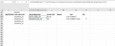
Stacking multiple FILTER results

[Lyonsyboy]

Hi
I have a FILTER array which lists multiple results from another Table (Column J). These have associated results that I would like to dynamically expand to list in a separate column (K). Is this possible?

Cheers

 

[jasonb75]

Try including both columns of the source table in the filter range.

 

[Lyonsyboy]

This is what I've had a crack at, but it only expands the top result....

Tried using J35# but it doesn't like it much.

 

[Alex Blakenburg]

By only giving us images and not giving us any idea of what your table looks like, it makes it really hard to help you.
There are a couple of options in the below. The filter one is what @jasonb75 is referring to.

In the below I have assumed that the columns you need are not next to each other because it is much simpler if they are (you would not need 2 filters).

PS: it would also be good if you update your profile to show which version of Excel you are using. While it is clear in this instance due to the use of Filter it may not be in other posts you make, and the version can impact the solution.

Book2
	A	B	C	D	E	F	G	H	I	J	K	L	M	N	O
1	Date to Filter				Criteria >	assays		Using G2#			Using Filter and extracting non-adjacent columns
2	1	assays	C1					1	C1		1	C1
3	2	assays	C2					2	C2		2	C2
4	3		C3					4	C4		4	C4
5	4	assays	C4
6	5		C5
7	6		C6
8
Sheet1

Cell Formulas
Range	Formula
H2:H4	H2	=FILTER($A$2:$A$7,$B$2:$B$7=$F$1,"Not Assayed")
I2:I4	I2	=VLOOKUP(H2#,$A$2:$C$7,3,FALSE)
K2:L4	K2	=FILTER(FILTER($A$2:$C$7,$B$2:$B$7=$F$1,"Not Assayed"),{1,0,1})
Dynamic array formulas.

 

[Lyonsyboy]

Sorry I'm pretty terrible at this. This is the filtered table (facesummary) with the results I want to list :

Sheet 3

So I'm looking for any instance of 'subs returned' in the 'submission' column of the face summary table which would list the corresponding 'face' in column K of sheet 3.

Basically, if G (Facesummary table) matches J (Sheet 3), return the 'Face' value from (Facesummary table) A, in K (Sheet 3). The list in (Sheet 3) J changes daily.

 

[jasonb75]

One of these should do it (2 versions of the same formula for different scenarios).

If the list in J35:J38 is produced by another dynamic array formula then try this one.

=FILTER(FaceSummary[Face],ISNUMBER(XMATCH(FaceSummary[Submission],J35#)),"No matches")

If it is not then you would need this one

=FILTER(FaceSummary[Face],ISNUMBER(XMATCH(FaceSummary[Submission],J35:INDEX(J:J,XMATCH("zzz",J:J,-1)))),"No matches")

Hopefully no typos.